FIFA World Cup 2018

In this project, I did an analysis and some visualizations on the FIFA18 dataset. The dataset is collected at this GitHub Repo. The goal is to predict the best possible international squad lineups for these 10 teams France, Germany, Spain, England, Brazil, Argentina, Belgium, Portugal, Uruguay, and Croatia at the 2018 World Cup this summer in Russia.
Published on April 23, 2018 by Udbhav Pangotra
pandas numpy plotly matplotlib
345 min READ
The FIFA World Cup, often simply called the World Cup, is an international association football competition contested by the senior men’s national teams of the members of the Fédération Internationale de Football Association (FIFA), the sport’s global governing body. The championship has been awarded every four years since the inaugural tournament in 1930, except in 1942 and 1946 when it was not held because of the Second World War. The current champion is France, which won its second title at the 2018 tournament in Russia.
# Import libraries
# conda install plotly

import sys
!{sys.executable} -m pip install plotly==2.7.0
!{sys.executable} -m pip install geopy
import pandas as pd
import numpy as np

import seaborn as sns
import matplotlib.pyplot as plt
%matplotlib inline

from plotly.offline import iplot, init_notebook_mode
from geopy.geocoders import Nominatim
import plotly.plotly as py
Collecting plotly==2.7.0
  Using cached plotly-2.7.0.tar.gz (25.0 MB)
Requirement already satisfied: decorator>=4.0.6 in c:\users\udbha\anaconda3\lib\site-packages (from plotly==2.7.0) (4.4.2)
Requirement already satisfied: nbformat>=4.2 in c:\users\udbha\anaconda3\lib\site-packages (from plotly==2.7.0) (5.0.8)
Requirement already satisfied: pytz in c:\users\udbha\anaconda3\lib\site-packages (from plotly==2.7.0) (2020.1)
Requirement already satisfied: requests in c:\users\udbha\anaconda3\lib\site-packages (from plotly==2.7.0) (2.24.0)
Requirement already satisfied: six in c:\users\udbha\anaconda3\lib\site-packages (from plotly==2.7.0) (1.15.0)
Requirement already satisfied: ipython-genutils in c:\users\udbha\anaconda3\lib\site-packages (from nbformat>=4.2->plotly==2.7.0) (0.2.0)
Requirement already satisfied: traitlets>=4.1 in c:\users\udbha\anaconda3\lib\site-packages (from nbformat>=4.2->plotly==2.7.0) (5.0.5)
Requirement already satisfied: jupyter-core in c:\users\udbha\anaconda3\lib\site-packages (from nbformat>=4.2->plotly==2.7.0) (4.6.3)
Requirement already satisfied: jsonschema!=2.5.0,>=2.4 in c:\users\udbha\anaconda3\lib\site-packages (from nbformat>=4.2->plotly==2.7.0) (3.2.0)
Requirement already satisfied: certifi>=2017.4.17 in c:\users\udbha\anaconda3\lib\site-packages (from requests->plotly==2.7.0) (2020.6.20)
Requirement already satisfied: chardet<4,>=3.0.2 in c:\users\udbha\anaconda3\lib\site-packages (from requests->plotly==2.7.0) (3.0.4)
Requirement already satisfied: urllib3!=1.25.0,!=1.25.1,<1.26,>=1.21.1 in c:\users\udbha\anaconda3\lib\site-packages (from requests->plotly==2.7.0) (1.25.11)
Requirement already satisfied: idna<3,>=2.5 in c:\users\udbha\anaconda3\lib\site-packages (from requests->plotly==2.7.0) (2.10)
Requirement already satisfied: pywin32>=1.0; sys_platform == "win32" in c:\users\udbha\anaconda3\lib\site-packages (from jupyter-core->nbformat>=4.2->plotly==2.7.0) (227)
Requirement already satisfied: attrs>=17.4.0 in c:\users\udbha\anaconda3\lib\site-packages (from jsonschema!=2.5.0,>=2.4->nbformat>=4.2->plotly==2.7.0) (20.3.0)
Requirement already satisfied: pyrsistent>=0.14.0 in c:\users\udbha\anaconda3\lib\site-packages (from jsonschema!=2.5.0,>=2.4->nbformat>=4.2->plotly==2.7.0) (0.17.3)
Requirement already satisfied: setuptools in c:\users\udbha\anaconda3\lib\site-packages (from jsonschema!=2.5.0,>=2.4->nbformat>=4.2->plotly==2.7.0) (50.3.1.post20201107)
Building wheels for collected packages: plotly
  Building wheel for plotly (setup.py): started
  Building wheel for plotly (setup.py): finished with status 'done'
  Created wheel for plotly: filename=plotly-2.7.0-py3-none-any.whl size=25015302 sha256=094b495e6f334ea880eab5832bb6d4bc2617d86dadd7729deac8954dbd4da3cc
  Stored in directory: c:\users\udbha\appdata\local\pip\cache\wheels\c6\05\50\0fcb05ea8220a1165ba12231211f7920d7f0a524b66d772325
Successfully built plotly
Installing collected packages: plotly
Successfully installed plotly-2.7.0
Collecting geopy
  Using cached geopy-2.1.0-py3-none-any.whl (112 kB)
Collecting geographiclib<2,>=1.49
  Using cached geographiclib-1.50-py3-none-any.whl (38 kB)
Installing collected packages: geographiclib, geopy
Successfully installed geographiclib-1.50 geopy-2.1.0
1 - Data Preparation
1.1 Load Data
FIFA18 = pd.read_csv('CompleteDataset.csv', low_memory=False)
FIFA18.columns
Index(['Unnamed: 0', 'Name', 'Age', 'Photo', 'Nationality', 'Flag', 'Overall',
       'Potential', 'Club', 'Club Logo', 'Value', 'Wage', 'Special',
       'Acceleration', 'Aggression', 'Agility', 'Balance', 'Ball control',
       'Composure', 'Crossing', 'Curve', 'Dribbling', 'Finishing',
       'Free kick accuracy', 'GK diving', 'GK handling', 'GK kicking',
       'GK positioning', 'GK reflexes', 'Heading accuracy', 'Interceptions',
       'Jumping', 'Long passing', 'Long shots', 'Marking', 'Penalties',
       'Positioning', 'Reactions', 'Short passing', 'Shot power',
       'Sliding tackle', 'Sprint speed', 'Stamina', 'Standing tackle',
       'Strength', 'Vision', 'Volleys', 'CAM', 'CB', 'CDM', 'CF', 'CM', 'ID',
       'LAM', 'LB', 'LCB', 'LCM', 'LDM', 'LF', 'LM', 'LS', 'LW', 'LWB',
       'Preferred Positions', 'RAM', 'RB', 'RCB', 'RCM', 'RDM', 'RF', 'RM',
       'RS', 'RW', 'RWB', 'ST'],
      dtype='object')
Let’s select the most interesting columns from loaded dataset:
interesting_columns = [
    'Name',
    'Age',
    'Nationality',
    'Overall',
    'Potential',
    'Club',
    'Value',
    'Wage',
    'Preferred Positions'
]
FIFA18 = pd.DataFrame(FIFA18, columns=interesting_columns)
1.2 Summarize Data
FIFA18.head()
| Name | Age | Nationality | Overall | Potential | Club | Value | Wage | Preferred Positions | |
|---|---|---|---|---|---|---|---|---|---|
| 0 | Cristiano Ronaldo | 32 | Portugal | 94 | 94 | Real Madrid CF | €95.5M | €565K | ST LW |
| 1 | L. Messi | 30 | Argentina | 93 | 93 | FC Barcelona | €105M | €565K | RW |
| 2 | Neymar | 25 | Brazil | 92 | 94 | Paris Saint-Germain | €123M | €280K | LW |
| 3 | L. Suárez | 30 | Uruguay | 92 | 92 | FC Barcelona | €97M | €510K | ST |
| 4 | M. Neuer | 31 | Germany | 92 | 92 | FC Bayern Munich | €61M | €230K | GK |
FIFA18.info()
<class 'pandas.core.frame.DataFrame'>
RangeIndex: 17981 entries, 0 to 17980
Data columns (total 9 columns):
 #   Column               Non-Null Count  Dtype
---  ------               --------------  -----
 0   Name                 17981 non-null  object
 1   Age                  17981 non-null  int64
 2   Nationality          17981 non-null  object
 3   Overall              17981 non-null  int64
 4   Potential            17981 non-null  int64
 5   Club                 17733 non-null  object
 6   Value                17981 non-null  object
 7   Wage                 17981 non-null  object
 8   Preferred Positions  17981 non-null  object
dtypes: int64(3), object(6)
memory usage: 1.2+ MB
1.3 Preprocess Data
Right away I can see that values in columns: ‘Value’ and ‘Wage’ aren’t numeric but objects. Thus I’ll preprocess the data to make it usable. I will use short supporting function to convert values in those two columns into numbers. I will end up with two new columns ‘ValueNum’ and ‘WageNum’ that will contain numeric values.
# Supporting function for converting string values into numbers
def str2number(amount):
    if amount[-1] == 'M':
        return float(amount[1:-1])*1000000
    elif amount[-1] == 'K':
        return float(amount[1:-1])*1000
    else:
        return float(amount[1:])

FIFA18['ValueNum'] = FIFA18['Value'].apply(lambda x: str2number(x))
FIFA18['WageNum'] = FIFA18['Wage'].apply(lambda x: str2number(x))
To make things simpler, I select the first position from list as preferred and save it in ‘Position’ column.
FIFA18['Position'] = FIFA18['Preferred Positions'].str.split().str[0]
2 - Data Visualization
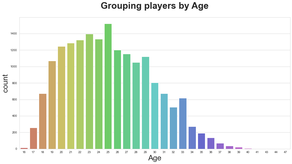
2.1 Age
plt.figure(figsize=(16,8))
sns.set_style("whitegrid")
plt.title('Grouping players by Age', fontsize=30, fontweight='bold', y=1.05,)
plt.xlabel('Number of players', fontsize=25)
plt.ylabel('Players Age', fontsize=25)
sns.countplot(x="Age", data=FIFA18, palette="hls");
plt.show()
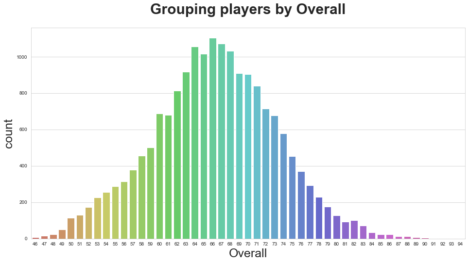
2.2 Overall
plt.figure(figsize=(16,8))
sns.set_style("whitegrid")
plt.title('Grouping players by Overall', fontsize=30, fontweight='bold', y=1.05,)
plt.xlabel('Number of players', fontsize=25)
plt.ylabel('Players Age', fontsize=25)
sns.countplot(x="Overall", data=FIFA18, palette="hls");
plt.show()
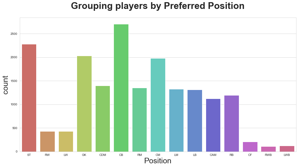
2.3 Preferred Position
plt.figure(figsize=(16,8))
sns.set_style("whitegrid")
plt.title('Grouping players by Preferred Position', fontsize=30, fontweight='bold', y=1.05,)
plt.xlabel('Number of players', fontsize=25)
plt.ylabel('Players Age', fontsize=25)
sns.countplot(x="Position", data=FIFA18, palette="hls");
plt.show()
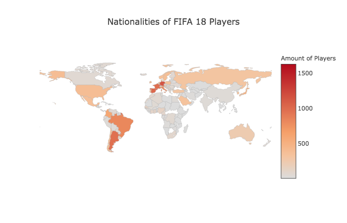
2.4 Nationality
In case the plot.ly image doesn’t show:
# Grouping the data by countries
valcon = FIFA18.groupby("Nationality").size().reset_index(name="Count")

# Plotting the choropleth map
init_notebook_mode()
plotmap = [ dict(
        type = 'choropleth',
        locations = valcon["Nationality"],
        locationmode = 'country names',
        z = valcon["Count"],
        text = valcon["Nationality"],
        autocolorscale = True,
        reversescale = False,
        marker = dict(
            line = dict (
                color = 'rgb(180,180,180)',
                width = 0.5
            ) ),
        colorbar = dict(
            title = "Amount of Players"),
      ) ]

layout = dict(
    # title = "Nationalities of FIFA 18 Players",
    geo = dict(
        # showframe = False,
        # showcoastlines = False,
        projection = dict(
            type = 'natural earth'
        )
    )
)

fig = dict( data=plotmap, layout=layout )
iplot(fig)
FIFA18["Nationality"].value_counts().head(25)
England                1630
Germany                1140
Spain                  1019
France                  978
Argentina               965
Brazil                  812
Italy                   799
Colombia                592
Japan                   469
Netherlands             429
Republic of Ireland     417
United States           381
Chile                   375
Sweden                  368
Portugal                367
Mexico                  360
Denmark                 346
Poland                  337
Norway                  333
Korea Republic          330
Saudi Arabia            329
Russia                  306
Scotland                300
Turkey                  291
Belgium                 272
Name: Nationality, dtype: int64
I can see that the players are very centralized in Europe. To be precise, England, Germany, Spain, and France.
2.5 Value
Let’s see the 20 players with highest value:
sorted_players = FIFA18.sort_values(["ValueNum"], ascending=False).head(20)
players = sorted_players[["Name" ,"Age" ,"Nationality" ,"Club" ,"Position" ,"Value"]].values
from IPython.display import HTML, display

table_content = ''
for row in players:
    HTML_row = '<tr>'
    HTML_row += '<td>' + str(row[0]) + '</td>'
    HTML_row += '<td>' + str(row[1]) + '</td>'
    HTML_row += '<td>' + str(row[2]) + '</td>'
    HTML_row += '<td>' + str(row[3]) + '</td>'
    HTML_row += '<td>' + str(row[4]) + '</td>'
    HTML_row += '<td>' + str(row[5]) + '</td>'

    table_content += HTML_row + '</tr>'

display(HTML(
    '<table><tr><th>Name</th><th>Age</th><th>Nationality</th><th>Club</th><th>Position</th><th>Value</th></tr>{}</table>'.format(table_content))
)
| Name | Age | Nationality | Club | Position | Value |
|---|---|---|---|---|---|
| Neymar | 25 | Brazil | Paris Saint-Germain | LW | €123M |
| L. Messi | 30 | Argentina | FC Barcelona | RW | €105M |
| L. Suárez | 30 | Uruguay | FC Barcelona | ST | €97M |
| Cristiano Ronaldo | 32 | Portugal | Real Madrid CF | ST | €95.5M |
| R. Lewandowski | 28 | Poland | FC Bayern Munich | ST | €92M |
| E. Hazard | 26 | Belgium | Chelsea | LW | €90.5M |
| K. De Bruyne | 26 | Belgium | Manchester City | RM | €83M |
| T. Kroos | 27 | Germany | Real Madrid CF | CDM | €79M |
| P. Dybala | 23 | Argentina | Juventus | ST | €79M |
| G. Higuaín | 29 | Argentina | Juventus | ST | €77M |
| A. Griezmann | 26 | France | Atlético Madrid | LW | €75M |
| Thiago | 26 | Spain | FC Bayern Munich | CDM | €70.5M |
| G. Bale | 27 | Wales | Real Madrid CF | RW | €69.5M |
| A. Sánchez | 28 | Chile | Arsenal | RM | €67.5M |
| S. Agüero | 29 | Argentina | Manchester City | ST | €66.5M |
| P. Pogba | 24 | France | Manchester United | CDM | €66.5M |
| C. Eriksen | 25 | Denmark | Tottenham Hotspur | LM | €65M |
| De Gea | 26 | Spain | Manchester United | GK | €64.5M |
| M. Verratti | 24 | Italy | Paris Saint-Germain | CDM | €64.5M |
| M. Neuer | 31 | Germany | FC Bayern Munich | GK | €61M |
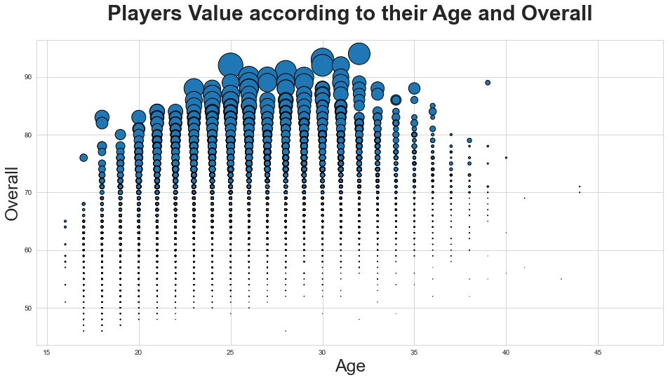
Let’s make a scatter chart of the players’ Value with respect to their Age and Overall:
plt.figure(figsize=(16,8))
sns.set_style("whitegrid")
plt.title('Players Value according to their Age and Overall', fontsize=30, fontweight='bold', y=1.05,)
plt.xlabel('Age', fontsize=25)
plt.ylabel('Overall', fontsize=25)

age = FIFA18["Age"].values
overall = FIFA18["Overall"].values
value = FIFA18["ValueNum"].values

plt.scatter(age, overall, s = value/100000, edgecolors='black')
plt.show()
2.6 Wage
Let’s see the 20 players with highest wage:
sorted_players = FIFA18.sort_values(["WageNum"], ascending=False).head(20)
players = sorted_players[["Name" ,"Age" ,"Nationality" ,"Club" ,"Position" ,"Wage"]].values
from IPython.display import HTML, display

table_content = ''
for row in players:
    HTML_row = '<tr>'
    HTML_row += '<td>' + str(row[0]) + '</td>'
    HTML_row += '<td>' + str(row[1]) + '</td>'
    HTML_row += '<td>' + str(row[2]) + '</td>'
    HTML_row += '<td>' + str(row[3]) + '</td>'
    HTML_row += '<td>' + str(row[4]) + '</td>'
    HTML_row += '<td>' + str(row[5]) + '</td>'

    table_content += HTML_row + '</tr>'

display(HTML(
    '<table><tr><th>Name</th><th>Age</th><th>Nationality</th><th>Club</th><th>Position</th><th>Wage</th></tr>{}</table>'.format(table_content))
)
| Name | Age | Nationality | Club | Position | Wage |
|---|---|---|---|---|---|
| Cristiano Ronaldo | 32 | Portugal | Real Madrid CF | ST | €565K |
| L. Messi | 30 | Argentina | FC Barcelona | RW | €565K |
| L. Suárez | 30 | Uruguay | FC Barcelona | ST | €510K |
| G. Bale | 27 | Wales | Real Madrid CF | RW | €370K |
| R. Lewandowski | 28 | Poland | FC Bayern Munich | ST | €355K |
| L. Modrić | 31 | Croatia | Real Madrid CF | CDM | €340K |
| T. Kroos | 27 | Germany | Real Madrid CF | CDM | €340K |
| S. Agüero | 29 | Argentina | Manchester City | ST | €325K |
| Sergio Ramos | 31 | Spain | Real Madrid CF | CB | €310K |
| E. Hazard | 26 | Belgium | Chelsea | LW | €295K |
| K. Benzema | 29 | France | Real Madrid CF | ST | €295K |
| K. De Bruyne | 26 | Belgium | Manchester City | RM | €285K |
| Neymar | 25 | Brazil | Paris Saint-Germain | LW | €280K |
| I. Rakitić | 29 | Croatia | FC Barcelona | CM | €275K |
| G. Higuaín | 29 | Argentina | Juventus | ST | €275K |
| A. Sánchez | 28 | Chile | Arsenal | RM | €265K |
| M. Özil | 28 | Germany | Arsenal | RW | €265K |
| Iniesta | 33 | Spain | FC Barcelona | LM | €260K |
| Marcelo | 29 | Brazil | Real Madrid CF | LB | €250K |
| J. Rodríguez | 25 | Colombia | FC Bayern Munich | RM | €250K |
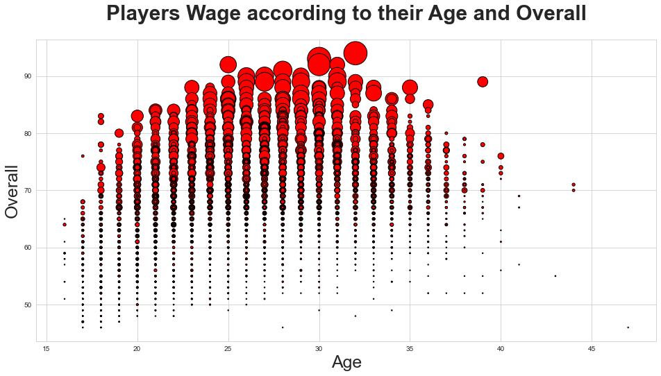
Let’s make a scatter chart of the players’ Wage with respect to their Age and Overall:
plt.figure(figsize=(16,8))
sns.set_style("whitegrid")
plt.title('Players Wage according to their Age and Overall', fontsize=30, fontweight='bold', y=1.05,)
plt.xlabel('Age', fontsize=25)
plt.ylabel('Overall', fontsize=25)

age = FIFA18["Age"].values
overall = FIFA18["Overall"].values
value = FIFA18["WageNum"].values

plt.scatter(age, overall, s = value/500, edgecolors='black', color="red")
plt.show()
3 - Best Squad Analysis
For simplicity of this analysis, I only pull in data I am interested in:
FIFA18 = FIFA18[['Name', 'Age', 'Nationality', 'Overall', 'Potential', 'Club', 'Position', 'Value', 'Wage']]
FIFA18.head(10)
| Name | Age | Nationality | Overall | Potential | Club | Position | Value | Wage | |
|---|---|---|---|---|---|---|---|---|---|
| 0 | Cristiano Ronaldo | 32 | Portugal | 94 | 94 | Real Madrid CF | ST | €95.5M | €565K |
| 1 | L. Messi | 30 | Argentina | 93 | 93 | FC Barcelona | RW | €105M | €565K |
| 2 | Neymar | 25 | Brazil | 92 | 94 | Paris Saint-Germain | LW | €123M | €280K |
| 3 | L. Suárez | 30 | Uruguay | 92 | 92 | FC Barcelona | ST | €97M | €510K |
| 4 | M. Neuer | 31 | Germany | 92 | 92 | FC Bayern Munich | GK | €61M | €230K |
| 5 | R. Lewandowski | 28 | Poland | 91 | 91 | FC Bayern Munich | ST | €92M | €355K |
| 6 | De Gea | 26 | Spain | 90 | 92 | Manchester United | GK | €64.5M | €215K |
| 7 | E. Hazard | 26 | Belgium | 90 | 91 | Chelsea | LW | €90.5M | €295K |
| 8 | T. Kroos | 27 | Germany | 90 | 90 | Real Madrid CF | CDM | €79M | €340K |
| 9 | G. Higuaín | 29 | Argentina | 90 | 90 | Juventus | ST | €77M | €275K |
3.1 Squad of Highest Overall Players
What’s the best squad according to FIFA 18 purely based on overall rating?
def get_best_squad(formation):
    FIFA18_copy = FIFA18.copy()
    store = []

    # iterate through all positions in the input formation and get players with highest overall respective to the position
    for i in formation:
        store.append([
            i,
            FIFA18_copy.loc[[FIFA18_copy[FIFA18_copy['Position'] == i]['Overall'].idxmax()]]['Name'].to_string(index = False),
            FIFA18_copy[FIFA18_copy['Position'] == i]['Overall'].max(),
            FIFA18_copy.loc[[FIFA18_copy[FIFA18_copy['Position'] == i]['Overall'].idxmax()]]['Age'].to_string(index = False),
            FIFA18_copy.loc[[FIFA18_copy[FIFA18_copy['Position'] == i]['Overall'].idxmax()]]['Club'].to_string(index = False),
            FIFA18_copy.loc[[FIFA18_copy[FIFA18_copy['Position'] == i]['Overall'].idxmax()]]['Value'].to_string(index = False),
            FIFA18_copy.loc[[FIFA18_copy[FIFA18_copy['Position'] == i]['Overall'].idxmax()]]['Wage'].to_string(index = False)
        ])

        FIFA18_copy.drop(FIFA18_copy[FIFA18_copy['Position'] == i]['Overall'].idxmax(),
                         inplace = True)

    # return store with only necessary columns
    return pd.DataFrame(np.array(store).reshape(11,7),
                        columns = ['Position', 'Player', 'Overall', 'Age', 'Club', 'Value', 'Wage']).to_string(index = False)
# 4-3-3
squad_433 = ['GK', 'RB', 'CB', 'CB', 'LB', 'CDM', 'CM', 'CAM', 'RW', 'ST', 'LW']
print ('4-3-3')
print (get_best_squad(squad_433))
4-3-3
Position              Player Overall  Age                  Club    Value    Wage
      GK            M. Neuer      92   31      FC Bayern Munich     €61M   €230K
      RB            Carvajal      84   25        Real Madrid CF     €32M   €195K
      CB        Sergio Ramos      90   31        Real Madrid CF     €52M   €310K
      CB        G. Chiellini      89   32              Juventus     €38M   €225K
      LB             Marcelo      87   29        Real Madrid CF     €38M   €250K
     CDM            T. Kroos      90   27        Real Madrid CF     €79M   €340K
      CM            N. Kanté      87   26               Chelsea   €52.5M   €190K
     CAM            Coutinho      86   25             Liverpool     €56M   €205K
      RW            L. Messi      93   30          FC Barcelona    €105M   €565K
      ST   Cristiano Ronaldo      94   32        Real Madrid CF   €95.5M   €565K
      LW              Neymar      92   25   Paris Saint-Germain    €123M   €280K
# 4-4-2
squad_442 = ['GK', 'RB', 'CB', 'CB', 'LB', 'RM', 'CM', 'CM', 'LM', 'ST', 'ST']
print ('4-4-2')
print (get_best_squad(squad_442))
4-4-2
Position              Player Overall  Age                Club    Value    Wage
      GK            M. Neuer      92   31    FC Bayern Munich     €61M   €230K
      RB            Carvajal      84   25      Real Madrid CF     €32M   €195K
      CB        Sergio Ramos      90   31      Real Madrid CF     €52M   €310K
      CB        G. Chiellini      89   32            Juventus     €38M   €225K
      LB             Marcelo      87   29      Real Madrid CF     €38M   €250K
      RM        K. De Bruyne      89   26     Manchester City     €83M   €285K
      CM            N. Kanté      87   26             Chelsea   €52.5M   €190K
      CM            A. Vidal      87   30    FC Bayern Munich   €37.5M   €160K
      LM          C. Eriksen      87   25   Tottenham Hotspur     €65M   €165K
      ST   Cristiano Ronaldo      94   32      Real Madrid CF   €95.5M   €565K
      ST           L. Suárez      92   30        FC Barcelona     €97M   €510K
# 4-2-3-1
squad_4231 = ['GK', 'RB', 'CB', 'CB', 'LB', 'CDM', 'CDM', 'CAM', 'CAM', 'CAM', 'ST']
print ('4-2-3-1')
print (get_best_squad(squad_4231))
4-2-3-1
Position              Player Overall  Age               Club    Value    Wage
      GK            M. Neuer      92   31   FC Bayern Munich     €61M   €230K
      RB            Carvajal      84   25     Real Madrid CF     €32M   €195K
      CB        Sergio Ramos      90   31     Real Madrid CF     €52M   €310K
      CB        G. Chiellini      89   32           Juventus     €38M   €225K
      LB             Marcelo      87   29     Real Madrid CF     €38M   €250K
     CDM            T. Kroos      90   27     Real Madrid CF     €79M   €340K
     CDM           L. Modrić      89   31     Real Madrid CF     €57M   €340K
     CAM            Coutinho      86   25          Liverpool     €56M   €205K
     CAM       R. Nainggolan      86   29               Roma   €42.5M   €130K
     CAM       Cesc Fàbregas      86   30            Chelsea     €41M   €210K
      ST   Cristiano Ronaldo      94   32     Real Madrid CF   €95.5M   €565K
Alright, now let’s move onto studying different squad’s impact on Nationality teams. First let’s modifiy above get_summary and get_best_squad functions for Nationality:
def get_best_squad_n(formation, nationality, measurement = 'Overall'):
    FIFA18_copy = FIFA18.copy()
    FIFA18_copy = FIFA18_copy[FIFA18_copy['Nationality'] == nationality]
    store = []

    for i in formation:
        store.append([
            FIFA18_copy.loc[[FIFA18_copy[FIFA18_copy['Position'].str.contains(i)][measurement].idxmax()]]['Position'].to_string(index = False),
            FIFA18_copy.loc[[FIFA18_copy[FIFA18_copy['Position'].str.contains(i)][measurement].idxmax()]]['Name'].to_string(index = False),
            FIFA18_copy[FIFA18_copy['Position'].str.contains(i)][measurement].max(),
            FIFA18_copy.loc[[FIFA18_copy[FIFA18_copy['Position'].str.contains(i)][measurement].idxmax()]]['Age'].to_string(index = False),
            FIFA18_copy.loc[[FIFA18_copy[FIFA18_copy['Position'].str.contains(i)][measurement].idxmax()]]['Club'].to_string(index = False),
            FIFA18_copy.loc[[FIFA18_copy[FIFA18_copy['Position'].str.contains(i)][measurement].idxmax()]]['Value'].to_string(index = False),
            FIFA18_copy.loc[[FIFA18_copy[FIFA18_copy['Position'].str.contains(i)][measurement].idxmax()]]['Wage'].to_string(index = False)
        ])

        FIFA18_copy.drop(FIFA18_copy[FIFA18_copy['Position'].str.contains(i)][measurement].idxmax(),
                         inplace = True)

    return np.mean([x[2] for x in store]).round(2), pd.DataFrame(np.array(store).reshape(11,7),
                                                                 columns = ['Position', 'Player', measurement, 'Age', 'Club', 'Value', 'Wage']).to_string(index = False)
def get_summary_n(squad_list, squad_name, nationality_list):
    summary = []

    for i in nationality_list:
        count = 0
        for j in squad_list:

            # for overall rating
            O_temp_rating, _  = get_best_squad_n(formation = j, nationality = i, measurement = 'Overall')

            # for potential rating & corresponding value
            P_temp_rating, _ = get_best_squad_n(formation = j, nationality = i, measurement = 'Potential')

            summary.append([i, squad_name[count], O_temp_rating.round(2), P_temp_rating.round(2)])
            count += 1

    return summary
Also let’s make our squad choices more strict:
squad_343_strict = ['GK', 'CB', 'CB', 'CB', 'RB|RWB', 'CM|CDM', 'CM|CDM', 'LB|LWB', 'RM|RW', 'ST|CF', 'LM|LW']
squad_442_strict = ['GK', 'RB|RWB', 'CB', 'CB', 'LB|LWB', 'RM', 'CM|CDM', 'CM|CAM', 'LM', 'ST|CF', 'ST|CF']
squad_4312_strict = ['GK', 'RB|RWB', 'CB', 'CB', 'LB|LWB', 'CM|CDM', 'CM|CAM|CDM', 'CM|CAM|CDM', 'CAM|CF', 'ST|CF', 'ST|CF']
squad_433_strict = ['GK', 'RB|RWB', 'CB', 'CB', 'LB|LWB', 'CM|CDM', 'CM|CAM|CDM', 'CM|CAM|CDM', 'RM|RW', 'ST|CF', 'LM|LW']
squad_4231_strict = ['GK', 'RB|RWB', 'CB', 'CB', 'LB|LWB', 'CM|CDM', 'CM|CDM', 'RM|RW', 'CAM', 'LM|LW', 'ST|CF']
squad_list = [squad_343_strict, squad_442_strict, squad_4312_strict, squad_433_strict, squad_4231_strict]
squad_name = ['3-4-3', '4-4-2', '4-3-1-2', '4-3-3', '4-2-3-1']
3.2 France
Let’s explore different squad possibility of France and how it affects the ratings:
France = pd.DataFrame(np.array(get_summary_n(squad_list, squad_name, ['France'])).reshape(-1,4), columns = ['Nationality', 'Squad', 'Overall', 'Potential'])
France.set_index('Nationality', inplace = True)
France[['Overall', 'Potential']] = France[['Overall', 'Potential']].astype(float)

print (France)
               Squad  Overall  Potential
Nationality
France         3-4-3    84.55      89.55
France         4-4-2    84.00      89.91
France       4-3-1-2    84.55      89.64
France         4-3-3    84.64      89.91
France       4-2-3-1    84.55      89.91
So we can say that France has the best squard as 4-3-3 for the current squad; and 4-4-2, 4-3-3, and 4-2-3-1 for the future squad based on team ratings. Let’s check out the best 11 squad line-up of France in 4-3-3 for current rating as well as 4-4-2 for potential rating:
rating_433_FR_Overall, best_list_433_FR_Overall = get_best_squad_n(squad_433_strict, 'France', 'Overall')
print('-Overall-')
print('Average rating: {:.1f}'.format(rating_433_FR_Overall))
print(best_list_433_FR_Overall)
-Overall-
Average rating: 84.6
Position         Player Overall  Age                      Club    Value    Wage
      GK      H. Lloris      88   30         Tottenham Hotspur     €38M   €165K
      RB       K. Zouma      79   22                Stoke City     €15M    €96K
      CB      R. Varane      85   24            Real Madrid CF   €46.5M   €175K
      CB     A. Laporte      84   23   Athletic Club de Bilbao   €35.5M    €36K
      LB     L. Kurzawa      80   24       Paris Saint-Germain   €16.5M    €69K
      CM       N. Kanté      87   26                   Chelsea   €52.5M   €190K
     CDM       P. Pogba      87   24         Manchester United   €66.5M   €195K
      CM     B. Matuidi      85   30                  Juventus   €28.5M   €145K
      RM     F. Thauvin      82   24    Olympique de Marseille     €28M    €40K
      ST     K. Benzema      86   29            Real Madrid CF   €44.5M   €295K
      LW   A. Griezmann      88   26           Atlético Madrid     €75M   €150K
rating_442_FR_Potential, best_list_442_FR_Potential = get_best_squad_n(squad_442_strict, 'France', 'Potential')
print('-Potential-')
print('Average rating: {:.1f}'.format(rating_442_FR_Potential))
print(best_list_442_FR_Potential)
-Potential-
Average rating: 89.9
Position         Player Potential  Age                      Club    Value    Wage
      GK      A. Lafont        89   18               Toulouse FC   €11.5M    €10K
      RB       K. Zouma        86   22                Stoke City     €15M    €96K
      CB      R. Varane        92   24            Real Madrid CF   €46.5M   €175K
      CB     A. Laporte        89   23   Athletic Club de Bilbao   €35.5M    €36K
      LB   L. Hernández        88   21           Atlético Madrid   €13.5M    €36K
      RM        A. Pléa        86   24                  OGC Nice   €20.5M    €41K
     CDM       P. Pogba        92   24         Manchester United   €66.5M   €195K
     CAM     O. Dembélé        92   20              FC Barcelona     €40M   €150K
      LM       T. Lemar        91   21                 AS Monaco   €38.5M    €37K
      ST      K. Mbappé        94   18       Paris Saint-Germain   €41.5M    €31K
      ST     A. Martial        90   21         Manchester United     €33M   €115K

3.3 Germany
The holding champion is certainly a heavy candidate for this year’s 1st place:
Germany = pd.DataFrame(np.array(get_summary_n(squad_list, squad_name, ['Germany'])).reshape(-1,4), columns = ['Nationality', 'Squad', 'Overall', 'Potential'])
Germany.set_index('Nationality', inplace = True)
Germany[['Overall', 'Potential']] = Germany[['Overall', 'Potential']].astype(float)

print (Germany)
               Squad  Overall  Potential
Nationality
Germany        3-4-3    86.27      88.55
Germany        4-4-2    85.09      88.36
Germany      4-3-1-2    85.36      88.00
Germany        4-3-3    86.27      88.55
Germany      4-2-3-1    86.09      88.55
As you can see, Germany’s current ratings peak with either 3-4-3 or 4-3-3 formation; while those 2 plus 4-2-3-1 are their best options for the future. With that, I’ll show Germany’s best 11 squad with 4-3-3 for current ratings and 4-2-3-1 for potential ratings.
rating_433_GER_Overall, best_list_433_GER_Overall = get_best_squad_n(squad_433_strict, 'Germany', 'Overall')
print('-Overall-')
print('Average rating: {:.1f}'.format(rating_433_GER_Overall))
print(best_list_433_GER_Overall)
-Overall-
Average rating: 86.3
Position        Player Overall  Age                Club    Value    Wage
      GK      M. Neuer      92   31    FC Bayern Munich     €61M   €230K
      RB    A. Rüdiger      82   24             Chelsea   €24.5M   €105K
      CB    J. Boateng      88   28    FC Bayern Munich     €48M   €215K
      CB    M. Hummels      88   28    FC Bayern Munich     €48M   €215K
      LB     J. Hector      80   27          1. FC Köln     €14M    €42K
     CDM      T. Kroos      90   27      Real Madrid CF     €79M   €340K
     CDM   I. Gündoğan      85   26     Manchester City     €46M   €190K
     CDM    S. Khedira      84   30            Juventus     €29M   €160K
      RW       M. Özil      88   28             Arsenal     €60M   €265K
      ST     T. Müller      86   27    FC Bayern Munich   €47.5M   €190K
      LW       M. Reus      86   28   Borussia Dortmund     €45M   €120K
rating_4231_GER_Potential, best_list_4231_GER_Potential = get_best_squad_n(squad_4231_strict, 'Germany', 'Potential')
print('-Potential-')
print('Average rating: {:.1f}'.format(rating_4231_GER_Potential))
print(best_list_4231_GER_Potential)
-Potential-
Average rating: 88.5
Position        Player Potential  Age                  Club    Value    Wage
      GK      M. Neuer        92   31      FC Bayern Munich     €61M   €230K
      RB    A. Rüdiger        86   24               Chelsea   €24.5M   €105K
      CB       N. Süle        89   21      FC Bayern Munich   €30.5M    €78K
      CB    J. Boateng        88   28      FC Bayern Munich     €48M   €215K
      LB   B. Henrichs        86   20   Bayer 04 Leverkusen     €11M    €36K
     CDM      T. Kroos        90   27        Real Madrid CF     €79M   €340K
     CDM   L. Goretzka        88   22         FC Schalke 04     €30M    €46K
      RW       M. Özil        88   28               Arsenal     €60M   €265K
     CAM     J. Brandt        88   21   Bayer 04 Leverkusen     €22M    €49K
      LM       L. Sané        91   21       Manchester City   €34.5M   €125K
      CF    K. Havertz        88   18   Bayer 04 Leverkusen      €8M    €25K

3.4 Spain
How about our 2010’s winner?
Spain = pd.DataFrame(np.array(get_summary_n(squad_list, squad_name, ['Spain'])).reshape(-1,4), columns = ['Nationality', 'Squad', 'Overall', 'Potential'])
Spain.set_index('Nationality', inplace = True)
Spain[['Overall', 'Potential']] = Spain[['Overall', 'Potential']].astype(float)

print (Spain)
               Squad  Overall  Potential
Nationality
Spain          3-4-3    86.27      88.82
Spain          4-4-2    86.45      88.73
Spain        4-3-1-2    86.55      88.09
Spain          4-3-3    86.64      89.00
Spain        4-2-3-1    86.64      89.00
Well, Spain does best with either 4-3-3 or 4-2-3-1 for both current and potential rating. I’ll choose 4-2-3-1 for the current squad and 4-3-3 for the potential squad.
rating_4231_ESP_Overall, best_list_4231_ESP_Overall = get_best_squad_n(squad_4231_strict, 'Spain', 'Overall')
print('-Overall-')
print('Average rating: {:.1f}'.format(rating_4231_ESP_Overall))
print(best_list_4231_ESP_Overall)
-Overall-
Average rating: 86.6
Position            Player Overall  Age                Club    Value    Wage
      GK            De Gea      90   26   Manchester United   €64.5M   €215K
      RB          Carvajal      84   25      Real Madrid CF     €32M   €195K
      CB      Sergio Ramos      90   31      Real Madrid CF     €52M   €310K
      CB             Piqué      87   30        FC Barcelona   €37.5M   €240K
      LB        Jordi Alba      85   28        FC Barcelona   €30.5M   €215K
     CDM            Thiago      88   26    FC Bayern Munich   €70.5M   €225K
      CM   Sergio Busquets      86   28        FC Barcelona     €36M   €250K
      RM         Juan Mata      84   29   Manchester United   €30.5M   €195K
     CAM     Cesc Fàbregas      86   30             Chelsea     €41M   €210K
      LM       David Silva      87   31     Manchester City     €44M   €220K
      ST       Diego Costa      86   28             Chelsea     €46M   €235K
rating_433_ESP_Potential, best_list_433_ESP_Potential = get_best_squad_n(squad_433_strict, 'Spain', 'Potential')
print('-Potential-')
print('Average rating: {:.1f}'.format(rating_433_ESP_Potential))
print(best_list_433_ESP_Potential)
-Potential-
Average rating: 89.0
Position            Player Potential  Age                Club    Value    Wage
      GK            De Gea        92   26   Manchester United   €64.5M   €215K
      RB   Héctor Bellerín        88   22             Arsenal     €21M    €91K
      CB      Sergio Ramos        90   31      Real Madrid CF     €52M   €310K
      CB             Piqué        87   30        FC Barcelona   €37.5M   €240K
      LB       Azpilicueta        87   27             Chelsea   €37.5M   €160K
     CDM            Thiago        90   26    FC Bayern Munich   €70.5M   €225K
     CAM     Dani Ceballos        88   20      Real Madrid CF   €16.5M   €105K
     CDM    Diego Llorente        87   23       Real Sociedad     €16M    €29K
      RM              Saúl        90   22     Atlético Madrid     €32M    €59K
      ST            Morata        88   24             Chelsea     €41M   €170K
      LW     Marco Asensio        92   21      Real Madrid CF     €46M   €175K

3.5 England
Although having the best soccer league in Europe, England did not seem to do that well at the national level. Let’s figure out their options for the upcoming World Cup:
England = pd.DataFrame(np.array(get_summary_n(squad_list, squad_name, ['England'])).reshape(-1,4), columns = ['Nationality', 'Squad', 'Overall', 'Potential'])
England.set_index('Nationality', inplace = True)
England[['Overall', 'Potential']] = England[['Overall', 'Potential']].astype(float)

print (England)
               Squad  Overall  Potential
Nationality
England        3-4-3    82.64      87.18
England        4-4-2    82.64      87.27
England      4-3-1-2    82.27      86.73
England        4-3-3    82.73      87.36
England      4-2-3-1    82.36      87.36
England should stick to 4-3-3 with their current squad and either 4-3-3 or 4-2-3-1 with their potential squad. Thus, I’ll choose 4-3-3 and 4-2-3-1 respectively.
rating_433_ENG_Overall, best_list_433_ENG_Overall = get_best_squad_n(squad_433_strict, 'England', 'Overall')
print('-Overall-')
print('Average rating: {:.1f}'.format(rating_433_ENG_Overall))
print(best_list_433_ENG_Overall)
-Overall-
Average rating: 82.7
Position         Player Overall  Age                Club    Value    Wage
      GK        J. Hart      82   30     West Ham United     €14M   €110K
     RWB      K. Walker      83   27     Manchester City     €24M   €130K
      CB      G. Cahill      84   31             Chelsea     €21M   €160K
      CB       M. Keane      81   24             Everton     €21M    €91K
     LWB        D. Rose      82   26   Tottenham Hotspur     €21M    €99K
      CM     A. Lallana      83   29           Liverpool     €25M   €135K
      CM        E. Dier      82   23   Tottenham Hotspur     €25M    €85K
      CM   J. Henderson      82   27           Liverpool   €21.5M   €115K
      RW     R. Barkley      81   23             Everton     €24M   €105K
      ST        H. Kane      86   23   Tottenham Hotspur     €59M   €165K
      LM        D. Alli      84   21   Tottenham Hotspur     €43M   €115K
rating_4231_ENG_Potential, best_list_4231_ENG_Potential = get_best_squad_n(squad_4231_strict, 'England', 'Potential')
print('-Potential-')
print('Average rating: {:.1f}'.format(rating_4231_ENG_Potential))
print(best_list_4231_ENG_Potential)
-Potential-
Average rating: 87.4
Position                  Player Potential  Age                Club    Value    Wage
      GK              J. Butland        87   24          Stoke City     €18M    €50K
     RWB   A. Oxlade-Chamberlain        85   23           Liverpool     €20M   €105K
      CB                M. Keane        87   24             Everton     €21M    €91K
      CB               J. Stones        85   23     Manchester City   €14.5M   €105K
      LB                 L. Shaw        84   21   Manchester United     €14M    €91K
      CM                A. Gomes        90   16   Manchester United    €975K     €9K
      CM                 E. Dier        87   23   Tottenham Hotspur     €25M    €85K
      RM             M. Rashford        89   19   Manchester United     €22M    €74K
     CAM              M. Edwards        87   18   Tottenham Hotspur    €1.2M    €11K
      LM                 D. Alli        90   21   Tottenham Hotspur     €43M   €115K
      ST                 H. Kane        90   23   Tottenham Hotspur     €59M   €165K

3.6 Brazil
Having won the World Cup the most times in history, the Samba team will no doubt be one of the top candidates for this summer in Russia.
Brazil = pd.DataFrame(np.array(get_summary_n(squad_list, squad_name, ['Brazil'])).reshape(-1,4), columns = ['Nationality', 'Squad', 'Overall', 'Potential'])
Brazil.set_index('Nationality', inplace = True)
Brazil[['Overall', 'Potential']] = Brazil[['Overall', 'Potential']].astype(float)

print (Brazil)
               Squad  Overall  Potential
Nationality
Brazil         3-4-3    85.36      88.45
Brazil         4-4-2    84.73      88.00
Brazil       4-3-1-2    84.64      88.00
Brazil         4-3-3    85.45      88.73
Brazil       4-2-3-1    85.36      88.73
As you can see, Brazil has similar options like England. I’ll go with 4-3-3 for the current rating and 4-2-3-1 for the potential rating.
rating_433_BRA_Overall, best_list_433_BRA_Overall = get_best_squad_n(squad_433_strict, 'Brazil', 'Overall')
print('-Overall-')
print('Average rating: {:.1f}'.format(rating_433_BRA_Overall))
print(best_list_433_BRA_Overall)
-Overall-
Average rating: 85.5
Position          Player Overall  Age                  Club    Value    Wage
      GK         Ederson      83   23       Manchester City     €26M    €87K
      RB      Dani Alves      84   34   Paris Saint-Germain      €9M   €115K
      CB    Thiago Silva      88   32   Paris Saint-Germain     €34M   €175K
      CB      David Luiz      86   30               Chelsea     €33M   €190K
      LB         Marcelo      87   29        Real Madrid CF     €38M   €250K
     CDM        Casemiro      85   25        Real Madrid CF     €42M   €195K
     CAM        Coutinho      86   25             Liverpool     €56M   €205K
     CAM         Willian      84   28               Chelsea   €31.5M   €200K
      RM   Douglas Costa      82   26              Juventus     €24M   €115K
      CF           Jonas      83   33            SL Benfica   €16.5M    €21K
      LW          Neymar      92   25   Paris Saint-Germain    €123M   €280K
rating_4231_BRA_Potential, best_list_4231_BRA_Potential = get_best_squad_n(squad_4231_strict, 'Brazil', 'Potential')
print('-Potential-')
print('Average rating: {:.1f}'.format(rating_4231_BRA_Potential))
print(best_list_4231_BRA_Potential)
-Potential-
Average rating: 88.7
Position          Player Potential  Age                    Club    Value    Wage
      GK         Ederson        89   23         Manchester City     €26M    €87K
      RB      Dani Alves        84   34     Paris Saint-Germain      €9M   €115K
      CB      Marquinhos        89   23     Paris Saint-Germain   €30.5M    €75K
      CB    Thiago Silva        88   32     Paris Saint-Germain     €34M   €175K
      LB         Marcelo        87   29          Real Madrid CF     €38M   €250K
     CDM        Casemiro        89   25          Real Madrid CF     €42M   €195K
     CDM         Fabinho        88   23               AS Monaco   €29.5M    €37K
      RM          Malcom        87   20   Girondins de Bordeaux   €24.5M    €47K
     CAM        Coutinho        89   25               Liverpool     €56M   €205K
      LW          Neymar        94   25     Paris Saint-Germain    €123M   €280K
      ST   Gabriel Jesus        92   20         Manchester City     €31M   €115K

3.7 Argentina
Lionel Messi is still waiting for the only trophy he hasn’t gotten yet in his career. Can he carry Argentina to the top after going short in the final 4 years ago?
Argentina = pd.DataFrame(np.array(get_summary_n(squad_list, squad_name, ['Argentina'])).reshape(-1,4), columns = ['Nationality', 'Squad', 'Overall', 'Potential'])
Argentina.set_index('Nationality', inplace = True)
Argentina[['Overall', 'Potential']] = Argentina[['Overall', 'Potential']].astype(float)

print (Argentina)
               Squad  Overall  Potential
Nationality
Argentina      3-4-3    84.27      87.36
Argentina      4-4-2    83.45      87.27
Argentina    4-3-1-2    83.55      86.73
Argentina      4-3-3    84.27      87.36
Argentina    4-2-3-1    84.00      87.09
Both 3-4-3 and 4-3-3 fare very well for the current and potential ratings of Argentine players. For the sake of diversity, I’ll choose 3-4-3 for their current squad and 4-3-3 for their future squad.
rating_343_ARG_Overall, best_list_343_ARG_Overall = get_best_squad_n(squad_343_strict, 'Argentina', 'Overall')
print('-Overall-')
print('Average rating: {:.1f}'.format(rating_343_ARG_Overall))
print(best_list_343_ARG_Overall)
-Overall-
Average rating: 84.3
Position         Player Overall  Age                  Club    Value    Wage
      GK       G. Rulli      83   25         Real Sociedad   €25.5M    €28K
      CB    N. Otamendi      83   29       Manchester City     €20M   €140K
      CB   M. Musacchio      83   26                 Milan     €27M   €105K
      CB       E. Garay      83   30           Valencia CF     €19M    €40K
      RB    P. Zabaleta      79   32       West Ham United      €7M    €99K
      CM      E. Banega      83   29            Sevilla FC   €25.5M    €27K
      CM      L. Biglia      83   31                 Milan   €17.5M   €105K
      LB        M. Rojo      82   27     Manchester United     €21M   €130K
      RW       L. Messi      93   30          FC Barcelona    €105M   €565K
      ST     G. Higuaín      90   29              Juventus     €77M   €275K
      LW    A. Di María      85   29   Paris Saint-Germain   €37.5M   €145K
rating_433_ARG_Potential, best_list_433_ARG_Potential = get_best_squad_n(squad_433_strict, 'Argentina', 'Potential')
print('-Potential-')
print('Average rating: {:.1f}'.format(rating_433_ARG_Potential))
print(best_list_433_ARG_Potential)
-Potential-
Average rating: 87.4
Position         Player Potential  Age                   Club    Value    Wage
      GK       G. Rulli        89   25          Real Sociedad   €25.5M    €28K
      RB       J. Figal        82   23          Independiente      €8M    €16K
      CB   M. Musacchio        86   26                  Milan     €27M   €105K
      CB     E. Mammana        86   21   Zenit St. Petersburg     €10M    €36K
      LB        M. Rojo        83   27      Manchester United     €21M   €130K
      CM       E. Barco        90   18          Independiente    €6.5M     €8K
      CM    G. Lo Celso        86   21    Paris Saint-Germain     €10M    €48K
     CDM   S. Ascacibar        86   20          VfB Stuttgart      €7M    €17K
      RW       L. Messi        93   30           FC Barcelona    €105M   €565K
      ST      P. Dybala        93   23               Juventus     €79M   €215K
      LM     M. Lanzini        87   24        West Ham United   €24.5M    €95K

3.8 Belgium
The Red Devils has some of the best players in English Premier League, but can’t never seem to make it far in the national level. Can Hazard and De Bruyne drive them far this time?
Belgium = pd.DataFrame(np.array(get_summary_n(squad_list, squad_name, ['Belgium'])).reshape(-1,4), columns = ['Nationality', 'Squad', 'Overall', 'Potential'])
Belgium.set_index('Nationality', inplace = True)
Belgium[['Overall', 'Potential']] = Belgium[['Overall', 'Potential']].astype(float)

print (Belgium)
               Squad  Overall  Potential
Nationality
Belgium        3-4-3    83.91      86.55
Belgium        4-4-2    83.36      86.73
Belgium      4-3-1-2    83.09      86.09
Belgium        4-3-3    84.27      87.27
Belgium      4-2-3-1    84.00      87.00
Again, 4-3-3 is the best formation for Belgium’s both current and future squad.
rating_433_BEL_Overall, best_list_433_BEL_Overall = get_best_squad_n(squad_433_strict, 'Belgium', 'Overall')
print('-Overall-')
print('Average rating: {:.1f}'.format(rating_433_BEL_Overall))
print(best_list_433_BEL_Overall)
-Overall-
Average rating: 84.3
Position            Player Overall  Age                Club    Value    Wage
      GK       T. Courtois      89   25             Chelsea     €59M   €190K
      RB          T. Foket      73   22            KAA Gent    €5.5M    €19K
      CB   T. Alderweireld      86   28   Tottenham Hotspur   €40.5M   €165K
      CB     J. Vertonghen      85   30   Tottenham Hotspur   €28.5M   €130K
      LB      T. Vermaelen      78   31        FC Barcelona      €7M   €120K
     CDM        M. Dembélé      83   29   Tottenham Hotspur     €25M   €115K
     CAM     R. Nainggolan      86   29                Roma   €42.5M   €130K
     CAM         A. Witsel      82   28                 NaN       €0      €0
      RM      K. De Bruyne      89   26     Manchester City     €83M   €285K
      ST         R. Lukaku      86   24   Manchester United     €59M   €210K
      LW         E. Hazard      90   26             Chelsea   €90.5M   €295K
rating_433_BEL_Potential, best_list_433_BEL_Potential = get_best_squad_n(squad_433_strict, 'Belgium', 'Potential')
print('-Potential-')
print('Average rating: {:.1f}'.format(rating_433_BEL_Potential))
print(best_list_433_BEL_Potential)
-Potential-
Average rating: 87.3
Position            Player Potential  Age                Club    Value    Wage
      GK       T. Courtois        92   25             Chelsea     €59M   €190K
      RB          T. Foket        79   22            KAA Gent    €5.5M    €19K
      CB   T. Alderweireld        87   28   Tottenham Hotspur   €40.5M   €165K
      CB     L. Dendoncker        86   22      RSC Anderlecht     €15M    €25K
      LB         J. Lukaku        83   22               Lazio     €10M    €39K
      CM           D. Rigo        84   18                 PSV    €1.3M     €3K
     CAM      Y. Tielemans        90   20           AS Monaco   €23.5M    €35K
     CAM     R. Nainggolan        86   29                Roma   €42.5M   €130K
      RM      K. De Bruyne        92   26     Manchester City     €83M   €285K
      ST         R. Lukaku        90   24   Manchester United     €59M   €210K
      LW         E. Hazard        91   26             Chelsea   €90.5M   €295K

3.9 - Portugal
The winner of Euro 2016 and the best player in the world 3 times in a row, Cristiano Ronaldo, has a real chance in this tournament as well.
Portugal = pd.DataFrame(np.array(get_summary_n(squad_list, squad_name, ['Portugal'])).reshape(-1,4), columns = ['Nationality', 'Squad', 'Overall', 'Potential'])
Portugal.set_index('Nationality', inplace = True)
Portugal[['Overall', 'Potential']] = Portugal[['Overall', 'Potential']].astype(float)

print (Portugal)
               Squad  Overall  Potential
Nationality
Portugal       3-4-3    83.00      87.00
Portugal       4-4-2    83.00      87.27
Portugal     4-3-1-2    82.82      86.55
Portugal       4-3-3    83.45      87.45
Portugal     4-2-3-1    83.45      87.27
OK, I’ll go with 4-2-3-1 for current rating and 4-3-3 for potential rating of Portugal.
rating_4231_POR_Overall, best_list_4231_POR_Overall = get_best_squad_n(squad_4231_strict, 'Portugal', 'Overall')
print('-Overall-')
print('Average rating: {:.1f}'.format(rating_4231_POR_Overall))
print(best_list_4231_POR_Overall)
-Overall-
Average rating: 83.5
Position              Player Overall  Age                 Club    Value    Wage
      GK            A. Lopes      83   26   Olympique Lyonnais   €22.5M    €60K
      RB       Nélson Semedo      81   23         FC Barcelona   €20.5M   €125K
      CB                Pepe      86   34          Beşiktaş JK   €13.5M    €94K
      CB          José Fonte      79   33      West Ham United      €5M    €99K
      LB             Antunes      79   30            Getafe CF      €9M    €29K
      CM    William Carvalho      83   25          Sporting CP   €27.5M    €21K
      CM      Danilo Pereira      83   25             FC Porto   €27.5M    €18K
      RM      Bernardo Silva      84   22      Manchester City   €43.5M   €165K
     CAM          João Mário      83   24                Inter     €34M    €70K
      LM                Nani      83   30                Lazio   €24.5M    €47K
      ST   Cristiano Ronaldo      94   32       Real Madrid CF   €95.5M   €565K
rating_433_POR_Potential, best_list_433_POR_Potential = get_best_squad_n(squad_433_strict, 'Portugal', 'Potential')
print('-Potential-')
print('Average rating: {:.1f}'.format(rating_433_POR_Potential))
print(best_list_433_POR_Potential)
-Potential-
Average rating: 87.5
Position              Player Potential  Age                 Club    Value    Wage
      GK            A. Lopes        86   26   Olympique Lyonnais   €22.5M    €60K
      RB       Nélson Semedo        87   23         FC Barcelona   €20.5M   €125K
      CB                Pepe        86   34          Beşiktaş JK   €13.5M    €94K
      CB        Rúben Semedo        85   23        Villarreal CF   €12.5M    €27K
      LB         Rafa Soares        83   22               Fulham    €8.5M    €11K
      CM    William Carvalho        86   25          Sporting CP   €27.5M    €21K
     CAM          João Mário        88   24                Inter     €34M    €70K
     CAM         André Gomes        88   23         FC Barcelona     €30M   €150K
      RM      Bernardo Silva        91   22      Manchester City   €43.5M   €165K
      ST   Cristiano Ronaldo        94   32       Real Madrid CF   €95.5M   €565K
      LM      Gelson Martins        88   22          Sporting CP     €25M    €20K

3.10 - Uruguay
Uruguay has the 2 best strikers in Europe: Suarez & Cavani. Can they perform this time?
Uruguay = pd.DataFrame(np.array(get_summary_n(squad_list, squad_name, ['Uruguay'])).reshape(-1,4), columns = ['Nationality', 'Squad', 'Overall', 'Potential'])
Uruguay.set_index('Nationality', inplace = True)
Uruguay[['Overall', 'Potential']] = Uruguay[['Overall', 'Potential']].astype(float)

print (Uruguay)
               Squad  Overall  Potential
Nationality
Uruguay        3-4-3    80.64      84.91
Uruguay        4-4-2    81.09      85.27
Uruguay      4-3-1-2    81.09      84.73
Uruguay        4-3-3    80.18      84.91
Uruguay      4-2-3-1    79.82      84.27
Fantastic, Uruguay does best with a 4-3-1-2 for current rating and 4-4-2 for future rating.
rating_4312_URG_Overall, best_list_4312_URG_Overall = get_best_squad_n(squad_4312_strict, 'Uruguay', 'Overall')
print('-Overall-')
print('Average rating: {:.1f}'.format(rating_4312_URG_Overall))
print(best_list_4312_URG_Overall)
-Overall-
Average rating: 81.1
Position          Player Overall  Age                  Club    Value    Wage
      GK      F. Muslera      82   31        Galatasaray SK   €13.5M    €57K
      RB      M. Cáceres      77   30         Hellas Verona    €6.5M    €28K
      CB        D. Godín      88   31       Atlético Madrid     €40M   €125K
      CB      J. Giménez      83   22       Atlético Madrid   €28.5M    €53K
      LB        F. Ricca      74   22             Málaga CF      €7M    €18K
     CDM       M. Vecino      78   25                 Inter     €13M    €59K
     CDM        M. Lemos      77   21         UD Las Palmas   €10.5M    €17K
      CM   S. Cristóforo      76   23            Fiorentina    €8.5M    €48K
      CF      N. Lodeiro      78   28   Seattle Sounders FC   €10.5M    €11K
      ST       L. Suárez      92   30          FC Barcelona     €97M   €510K
      ST       E. Cavani      87   30   Paris Saint-Germain   €48.5M   €160K
rating_442_URG_Potential, best_list_442_URG_Potential = get_best_squad_n(squad_442_strict, 'Uruguay', 'Potential')
print('-Potential-')
print('Average rating: {:.1f}'.format(rating_442_URG_Potential))
print(best_list_442_URG_Potential)
-Potential-
Average rating: 85.3
Position        Player Potential  Age                        Club    Value    Wage
      GK    F. Muslera        82   31              Galatasaray SK   €13.5M    €57K
      RB   C. González        82   20            Sevilla Atlético    €1.8M     €3K
      CB      D. Godín        88   31             Atlético Madrid     €40M   €125K
      CB    J. Giménez        87   22             Atlético Madrid   €28.5M    €53K
     LWB   M. Saracchi        85   19                 River Plate    €3.4M     €7K
      RM   F. Valverde        85   18   RC Deportivo de La Coruña    €3.6M    €44K
      CM     N. Nández        85   21                Boca Juniors    €3.5M    €11K
      CM   L. Torreira        83   21                   Sampdoria     €10M    €26K
      LM     D. Laxalt        82   24                       Genoa   €13.5M    €30K
      ST     L. Suárez        92   30                FC Barcelona     €97M   €510K
      ST     E. Cavani        87   30         Paris Saint-Germain   €48.5M   €160K

3.11 - Croatia
Well, I’m a big fan of Modric and Rakitic. Needless to say about their winning habits?
Croatia = pd.DataFrame(np.array(get_summary_n(squad_list, squad_name, ['Croatia'])).reshape(-1,4), columns = ['Nationality', 'Squad', 'Overall', 'Potential'])
Croatia.set_index('Nationality', inplace = True)
Croatia[['Overall', 'Potential']] = Croatia[['Overall', 'Potential']].astype(float)

print (Croatia)
               Squad  Overall  Potential
Nationality
Croatia        3-4-3    80.55      83.00
Croatia        4-4-2    80.82      83.00
Croatia      4-3-1-2    81.27      83.64
Croatia        4-3-3    81.64      83.91
Croatia      4-2-3-1    81.64      83.64
Dope, Croatia is superior with a 4-2-3-1 using current form and 4-3-3 using potential form.
rating_4231_CRO_Overall, best_list_4231_CRO_Overall = get_best_squad_n(squad_4231_strict, 'Croatia', 'Overall')
print('-Overall-')
print('Average rating: {:.1f}'.format(rating_4231_CRO_Overall))
print(best_list_4231_CRO_Overall)
-Overall-
Average rating: 81.6
Position         Player Overall  Age               Club    Value    Wage
      GK     D. Subašić      85   32          AS Monaco     €22M    €46K
      RB        D. Srna      81   35   Shakhtar Donetsk    €3.8M     €1K
      CB     V. Ćorluka      82   31   Lokomotiv Moscow     €15M    €54K
      CB      D. Lovren      81   27          Liverpool   €17.5M   €110K
      LB     I. Strinić      75   29          Sampdoria      €5M    €31K
     CDM      L. Modrić      89   31     Real Madrid CF     €57M   €340K
      CM     I. Rakitić      87   29       FC Barcelona   €48.5M   €275K
      RM     J. Brekalo      70   19      VfB Stuttgart    €3.1M    €21K
     CAM     I. Perišić      84   28              Inter   €31.5M   €110K
      LM   M. Mandžukić      83   31           Juventus   €23.5M   €135K
      ST     N. Kalinić      81   29              Milan     €18M    €84K
rating_433_CRO_Potential, best_list_433_CRO_Potential = get_best_squad_n(squad_433_strict, 'Croatia', 'Potential')
print('-Potential-')
print('Average rating: {:.1f}'.format(rating_433_CRO_Potential))
print(best_list_433_CRO_Potential)
-Potential-
Average rating: 83.9
Position       Player Potential  Age                  Club    Value    Wage
      GK   D. Subašić        85   32             AS Monaco     €22M    €46K
      RB    T. Jedvaj        84   21   Bayer 04 Leverkusen     €10M    €36K
      CB    D. Lovren        83   27             Liverpool   €17.5M   €110K
      CB   V. Ćorluka        82   31      Lokomotiv Moscow     €15M    €54K
      LB     A. Milić        76   23           KV Oostende    €2.7M     €9K
     CDM    L. Modrić        89   31        Real Madrid CF     €57M   €340K
     CDM   M. Kovačić        88   23        Real Madrid CF     €30M   €150K
      CM   I. Rakitić        87   29          FC Barcelona   €48.5M   €275K
      RM   J. Brekalo        82   19         VfB Stuttgart    €3.1M    €21K
      ST   N. Kalinić        81   29                 Milan     €18M    €84K
      LW     M. Pjaca        86   22              Juventus   €12.5M    €89K

4 - Final Comparison
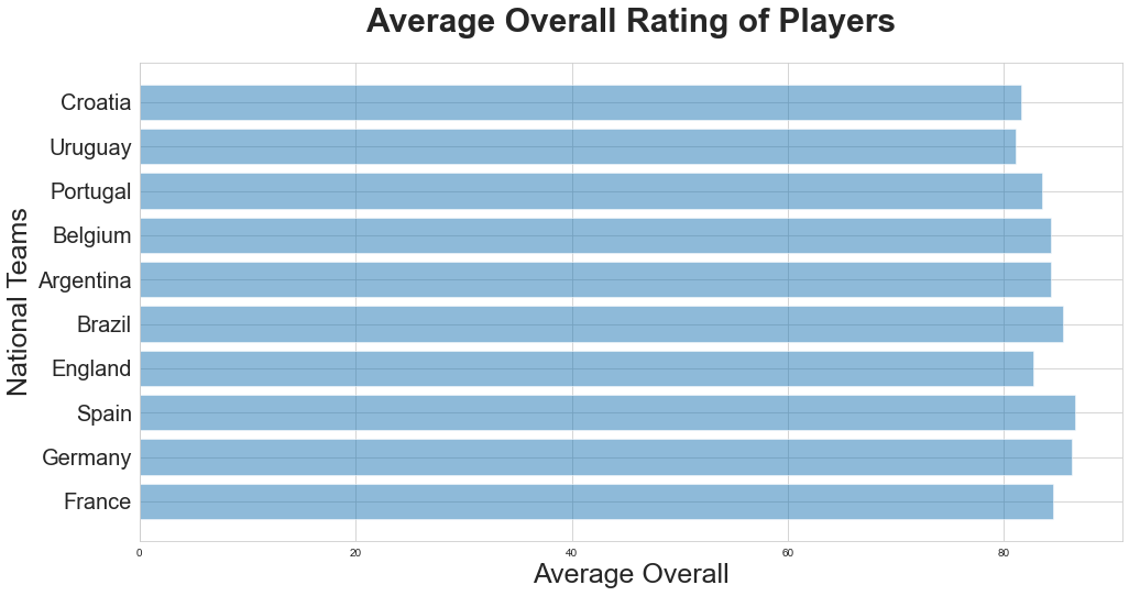
Ok, let’s make some comparison between these 10 line-ups with the current rating of players for these strongest contenders for World Cup 2018.
teams = ('France', 'Germany', 'Spain', 'England', 'Brazil', 'Argentina', 'Belgium', 'Portugal', 'Uruguay', 'Croatia')
index = np.arange(len(teams))
average_overall = [84.6, 86.3, 86.6, 82.7, 85.5, 84.3, 84.3, 83.5, 81.1, 81.6]

plt.figure(figsize=(16,8))
plt.barh(index, average_overall, align='center', alpha=0.5)
plt.yticks(index, teams, fontsize=20)
plt.ylabel('National Teams', fontsize=25)
plt.xlabel('Average Overall', fontsize=25)
plt.title('Average Overall Rating of Players', fontsize=30, fontweight='bold', y=1.05,)

plt.show()
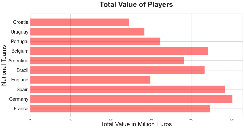
total_value = [446.5, 502, 484.5, 298.5, 433, 382, 440.5, 323, 283.5, 244.9]

plt.figure(figsize=(16,8))
plt.barh(index, total_value, align='center', alpha=0.5, color='red')
plt.yticks(index, teams, fontsize=20)
plt.ylabel('National Teams', fontsize=25)
plt.xlabel('Total Value in Million Euros', fontsize=25)
plt.title('Total Value of Players', fontsize=30, fontweight='bold', y=1.05,)

plt.show()
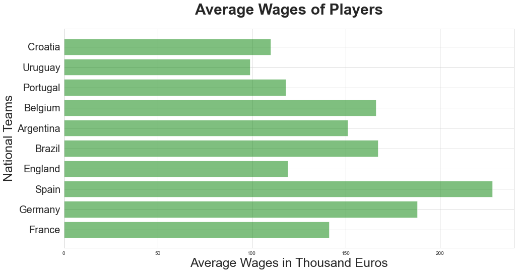
average_wage = [141, 188, 228, 119, 167, 151, 166, 118, 99, 110]

plt.figure(figsize=(16,8))
plt.barh(index, average_wage, align='center', alpha=0.5, color='green')
plt.yticks(index, teams, fontsize=20)
plt.ylabel('National Teams', fontsize=25)
plt.xlabel('Average Wages in Thousand Euros', fontsize=25)
plt.title('Average Wages of Players', fontsize=30, fontweight='bold', y=1.05,)

plt.show()
Conclusion
So based purely on the FIFA 18 Data:
- Spain has the highest average overall rating, followed by Germany and Brazil.
- Germany has the highest total value, followed by Spain and France.
- Spain has the highest average wage, followed by Germany and Brazil.
My bet is for a Spain vs France in the final, and Argentina vs Brazil for the 3rd place. Your turn?
- Also, this is personal but Portugal might just surprise us :P
- Hail Ronaldo!