Digit Recognizer

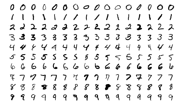
# MNIST ("Modified National Institute of Standards and Technology") is the de facto “hello world” dataset of computer vision. Since its release in 1999, this classic dataset of handwritten images has served as the basis for benchmarking classification algorithms. As new machine learning techniques emerge, MNIST remains a reliable resource for researchers and learners alike.


# This Python 3 environment comes with many helpful analytics libraries installed
# It is defined by the kaggle/python docker image: https://github.com/kaggle/docker-python
# For example, here's several helpful packages to load in 

import numpy as np # linear algebra
import pandas as pd # data processing, CSV file I/O (e.g. pd.read_csv)

# Input data files are available in the "../input/" directory.
# For example, running this (by clicking run or pressing Shift+Enter) will list all files under the input directory

import os
for dirname, _, filenames in os.walk('/kaggle/input'):
    for filename in filenames:
        print(os.path.join(dirname, filename))

# Any results you write to the current directory are saved as output.

train = pd.read_csv('/kaggle/input/digit-recognizer/train.csv')
test = pd.read_csv('/kaggle/input/digit-recognizer/test.csv')

import pandas as pd
import numpy as np
import matplotlib.pyplot as plt
import matplotlib.image as mpimg
import seaborn as sns
%matplotlib inline

np.random.seed(2)

from sklearn.model_selection import train_test_split
from sklearn.metrics import confusion_matrix
import itertools

from keras.utils.np_utils import to_categorical # convert to one-hot-encoding
from keras.models import Sequential
from keras.layers import Dense, Dropout, Flatten, Conv2D, MaxPool2D
from keras.optimizers import RMSprop
from keras.preprocessing.image import ImageDataGenerator
from keras.callbacks import ReduceLROnPlateau


sns.set(style='white', context='notebook', palette='deep')

Y_train = train["label"]
X_train = train.drop(labels = ["label"],axis = 1) 
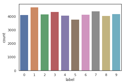
g = sns.countplot(Y_train)

Y_train.value_counts()

X_train.isna().any().sum(),test.isna().any().sum()

X_train=X_train/255
test=test/255

# Reshape image in 3 dimensions (height = 28px, width = 28px , canal = 1)
X_train = X_train.values.reshape(-1,28,28,1)
test = test.values.reshape(-1,28,28,1)

Y_train = to_categorical(Y_train, num_classes = 10)

random_seed = 2
X_train, X_val, Y_train, Y_val = train_test_split(X_train, Y_train, test_size = 0.1, random_state=random_seed)

X_train.shape

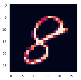
g = plt.imshow(X_train[0][:,:,0])

# Set the CNN model 
# my CNN architechture is In -> [[Conv2D->relu]*2 -> MaxPool2D -> Dropout]*2 -> Flatten -> Dense -> Dropout -> Out

model = Sequential()

model.add(Conv2D(filters = 32, kernel_size = (5,5),padding = 'Same', 
                 activation ='relu', input_shape = (28,28,1)))
model.add(Conv2D(filters = 32, kernel_size = (5,5),padding = 'Same', 
                 activation ='relu'))
model.add(MaxPool2D(pool_size=(2,2)))
model.add(Dropout(0.25))


model.add(Conv2D(filters = 64, kernel_size = (3,3),padding = 'Same', 
                 activation ='relu'))
model.add(Conv2D(filters = 64, kernel_size = (3,3),padding = 'Same', 
                 activation ='relu'))
model.add(MaxPool2D(pool_size=(2,2), strides=(2,2)))
model.add(Dropout(0.25))


model.add(Flatten())
model.add(Dense(256, activation = "relu"))
model.add(Dropout(0.5))
model.add(Dense(10, activation = "softmax"))

optimizer = RMSprop(lr=0.001, rho=0.9, epsilon=1e-08, decay=0.0)
model.compile(optimizer = optimizer , loss = "categorical_crossentropy", metrics=["accuracy"])

# Set a learning rate annealer
learning_rate_reduction = ReduceLROnPlateau(monitor='val_accuracy', 
                                            patience=3, 
                                            verbose=1, 
                                            factor=0.5, 
                                            min_lr=0.00001)

epochs = 50 # 
batch_size = 86

datagen = ImageDataGenerator(
        featurewise_center=False,  # set input mean to 0 over the dataset
        samplewise_center=False,  # set each sample mean to 0
        featurewise_std_normalization=False,  # divide inputs by std of the dataset
        samplewise_std_normalization=False,  # divide each input by its std
        zca_whitening=False,  # apply ZCA whitening
        rotation_range=10,  # randomly rotate images in the range (degrees, 0 to 180)
        zoom_range = 0.1, # Randomly zoom image 
        width_shift_range=0.1,  # randomly shift images horizontally (fraction of total width)
        height_shift_range=0.1,  # randomly shift images vertically (fraction of total height)
        horizontal_flip=False,  # randomly flip images
        vertical_flip=False)  # randomly flip images


datagen.fit(X_train)

# Fit the model
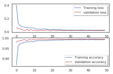
history = model.fit_generator(datagen.flow(X_train,Y_train, batch_size=batch_size),
                              epochs = epochs, validation_data = (X_val,Y_val),
                              verbose = 2, steps_per_epoch=X_train.shape[0] // batch_size
                              , callbacks=[learning_rate_reduction])

fig, ax = plt.subplots(2,1)
ax[0].plot(history.history['loss'], color='b', label="Training loss")
ax[0].plot(history.history['val_loss'], color='r', label="validation loss",axes =ax[0])
legend = ax[0].legend(loc='best', shadow=True)

ax[1].plot(history.history['accuracy'], color='b', label="Training accuracy")
ax[1].plot(history.history['val_accuracy'], color='r',label="Validation accuracy")
legend = ax[1].legend(loc='best', shadow=True)

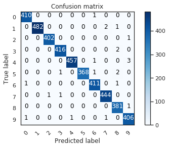
# Look at confusion matrix 

def plot_confusion_matrix(cm, classes,
                          normalize=False,
                          title='Confusion matrix',
                          cmap=plt.cm.Blues):
    """
    This function prints and plots the confusion matrix.
    Normalization can be applied by setting `normalize=True`.
    """
    plt.imshow(cm, interpolation='nearest', cmap=cmap)
    plt.title(title)
    plt.colorbar()
    tick_marks = np.arange(len(classes))
    plt.xticks(tick_marks, classes, rotation=45)
    plt.yticks(tick_marks, classes)

    if normalize:
        cm = cm.astype('float') / cm.sum(axis=1)[:, np.newaxis]

    thresh = cm.max() / 2.
    for i, j in itertools.product(range(cm.shape[0]), range(cm.shape[1])):
        plt.text(j, i, cm[i, j],
                 horizontalalignment="center",
                 color="white" if cm[i, j] > thresh else "black")

    plt.tight_layout()
    plt.ylabel('True label')
    plt.xlabel('Predicted label')

# Predict the values from the validation dataset
Y_pred = model.predict(X_val)
# Convert predictions classes to one hot vectors 
Y_pred_classes = np.argmax(Y_pred,axis = 1) 
# Convert validation observations to one hot vectors
Y_true = np.argmax(Y_val,axis = 1) 
# compute the confusion matrix
confusion_mtx = confusion_matrix(Y_true, Y_pred_classes) 
# plot the confusion matrix
plot_confusion_matrix(confusion_mtx, classes = range(10)) 

# predict results
results = model.predict(test)

# select the indix with the maximum probability
results = np.argmax(results,axis = 1)

results = pd.Series(results,name="Label")

submission = pd.concat([pd.Series(range(1,28001),name = "ImageId"),results],axis = 1)

submission.to_csv("cnn_mnist_datagen.csv",index=False)