Bitcoin Price Forecast

In this blog we work with time-series dataset consisting of bitcoin prices.
Published on January 05, 2021 by Udbhav Pangotra
pandas numpy plotly matplotlib Prophet
26 min READ
Bitcoin Historical Data Analysis
Bitcoin (₿) is a cryptocurrency invented in 2008 by an unknown person or group of people using the name Satoshi Nakamoto Some interesting facts about Bitcoin(BTC):
- Bitcoin is a decentralized digital currency, without a central bank or single administrator, that can be sent from user to user on the peer-to-peer bitcoin network without the need for intermediaries. Transactions are verified by network nodes through cryptography and recorded in a public distributed ledger called a blockchain.
- In fact, there are only 21 million bitcoins that can be mined in total.Once miners have unlocked this amount of bitcoins, the supply will be exhausted.
- Currently, around 18.5 million bitcoin have been mined. This leaves less than three million that have yet to be introduced into circulation.
#Data Pre-Processing packages:
import numpy as np
import pandas as pd
from datetime import datetime


#Data Visualization Packages:
#Seaborn
import seaborn as sns
sns.set(rc={'figure.figsize':(10,6)})
custom_colors = ["#4e89ae", "#c56183","#ed6663","#ffa372"]

#Matplotlib
import matplotlib.pyplot as plt
%matplotlib inline
import matplotlib.image as mpimg

#Colorama
from colorama import Fore, Back, Style # For text colors
y_= Fore.CYAN
m_= Fore.WHITE

#garbage collector - To free up unused space
import gc
gc.collect()

#NetworkX
import networkx as nx
import plotly.graph_objects as go #To construct network graphs

#To avoid printing of un necessary Deprecation warning and future warnings!
import warnings
warnings.filterwarnings("ignore", category=DeprecationWarning)
warnings.filterwarnings("ignore", category=FutureWarning)

#Time series Analysis pacakages:

from statsmodels.tsa.seasonal import seasonal_decompose
from statsmodels.tsa.stattools import kpss
from statsmodels.tsa.stattools import adfuller
from statsmodels.graphics.tsaplots import plot_acf, plot_pacf

#Facebook Prophet packages:
from fbprophet import Prophet
from fbprophet.diagnostics import cross_validation, performance_metrics
from fbprophet.plot import add_changepoints_to_plot, plot_cross_validation_metric

#Time -To find how long each cell takes to run
import time

#Importing of Data
data=pd.read_csv('../input/bitcoin-historical-data/bitstampUSD_1-min_data_2012-01-01_to_2020-12-31.csv')
Data set Overview & Pre-Processing
print(f"{m_}Total records:{y_}{data.shape}\n")
print(f"{m_}Data types of data columns: \n{y_}{data.dtypes}")
[37mTotal records:[36m(4727777, 8)
[37mData types of data columns:
[36mTimestamp int64
Open float64
High float64
Low float64
Close float64
Volume_(BTC) float64
Volume_(Currency) float64
Weighted_Price float64
dtype: object
Data Pre-processing steps
- Date
- Fill in the missing values interpolation
The data is available on a Hourly based on each day, So we need to resample them to day based.
data['Timestamp'] = [datetime.fromtimestamp(x) for x in data['Timestamp']]
data = data.set_index('Timestamp')
data = data.resample("24H").mean()
data.head()
| Open | High | Low | Close | Volume_(BTC) | Volume_(Currency) | Weighted_Price | |
|---|---|---|---|---|---|---|---|
| Timestamp | |||||||
| 2011-12-31 | 4.465000 | 4.482500 | 4.465000 | 4.482500 | 23.829470 | 106.330084 | 4.471603 |
| 2012-01-01 | 4.806667 | 4.806667 | 4.806667 | 4.806667 | 7.200667 | 35.259720 | 4.806667 |
| 2012-01-02 | 5.000000 | 5.000000 | 5.000000 | 5.000000 | 19.048000 | 95.240000 | 5.000000 |
| 2012-01-03 | 5.252500 | 5.252500 | 5.252500 | 5.252500 | 11.004660 | 58.100651 | 5.252500 |
| 2012-01-04 | 5.200000 | 5.223333 | 5.200000 | 5.223333 | 11.914807 | 63.119577 | 5.208159 |
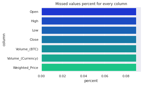
missed = pd.DataFrame()
missed['column'] = data.columns

missed['percent'] = [round(100* data[col].isnull().sum() / len(data), 2) for col in data.columns]
missed = missed.sort_values('percent',ascending=False)
missed = missed[missed['percent']>0]

fig = sns.barplot(
    x=missed['percent'],
    y=missed["column"],
    orientation='horizontal',palette="winter"
).set_title('Missed values percent for every column')
def fill_missing(df):
    ### function to impute missing values using interpolation ###
    df['Open'] = df['Open'].interpolate()
    df['Close'] = df['Close'].interpolate()
    df['Weighted_Price'] = df['Weighted_Price'].interpolate()
    df['Volume_(BTC)'] = df['Volume_(BTC)'].interpolate()
    df['Volume_(Currency)'] = df['Volume_(Currency)'].interpolate()
    df['High'] = df['High'].interpolate()
    df['Low'] = df['Low'].interpolate()
    print(f'{m_}No. of Missing values after interpolation:\n{y_}{df.isnull().sum()}')

fill_missing(data)
[37mNo. of Missing values after interpolation:
[36mOpen 0
High 0
Low 0
Close 0
Volume_(BTC) 0
Volume_(Currency) 0
Weighted_Price 0
dtype: int64
data.columns
Index(['Open', 'High', 'Low', 'Close', 'Volume_(BTC)', 'Volume_(Currency)',
       'Weighted_Price'],
      dtype='object')
new_df=data.groupby('Timestamp').mean()
new_df=new_df[['Volume_(BTC)', 'Close','Volume_(Currency)']]
new_df.rename(columns={'Volume_(BTC)':'Volume_market_mean','Close':'close_mean','Volume_(Currency)':'volume_curr_mean'},inplace=True)
new_df.head()
| Volume_market_mean | close_mean | volume_curr_mean | |
|---|---|---|---|
| Timestamp | |||
| 2011-12-31 | 23.829470 | 4.482500 | 106.330084 |
| 2012-01-01 | 7.200667 | 4.806667 | 35.259720 |
| 2012-01-02 | 19.048000 | 5.000000 | 95.240000 |
| 2012-01-03 | 11.004660 | 5.252500 | 58.100651 |
| 2012-01-04 | 11.914807 | 5.223333 | 63.119577 |
data_df = data.merge(new_df, left_on='Timestamp',
                                right_index=True)
data_df['volume(BTC)/Volume_market_mean'] = data_df['Volume_(BTC)'] / data_df['Volume_market_mean']
data_df['Volume_(Currency)/volume_curr_mean'] = data_df['Volume_(Currency)'] / data_df['volume_curr_mean']

data_df['close/close_market_mean'] = data_df['Close'] / data_df['close_mean']
data_df['open/close'] = data_df['Open'] / data_df['Close']
data_df["gap"] = data_df["High"] - data_df["Low"]
data_df.head()
| Open | High | Low | Close | Volume_(BTC) | Volume_(Currency) | Weighted_Price | Volume_market_mean | close_mean | volume_curr_mean | volume(BTC)/Volume_market_mean | Volume_(Currency)/volume_curr_mean | close/close_market_mean | open/close | gap | |
|---|---|---|---|---|---|---|---|---|---|---|---|---|---|---|---|
| Timestamp | |||||||||||||||
| 2011-12-31 | 4.465000 | 4.482500 | 4.465000 | 4.482500 | 23.829470 | 106.330084 | 4.471603 | 23.829470 | 4.482500 | 106.330084 | 1.0 | 1.0 | 1.0 | 0.996096 | 0.017500 |
| 2012-01-01 | 4.806667 | 4.806667 | 4.806667 | 4.806667 | 7.200667 | 35.259720 | 4.806667 | 7.200667 | 4.806667 | 35.259720 | 1.0 | 1.0 | 1.0 | 1.000000 | 0.000000 |
| 2012-01-02 | 5.000000 | 5.000000 | 5.000000 | 5.000000 | 19.048000 | 95.240000 | 5.000000 | 19.048000 | 5.000000 | 95.240000 | 1.0 | 1.0 | 1.0 | 1.000000 | 0.000000 |
| 2012-01-03 | 5.252500 | 5.252500 | 5.252500 | 5.252500 | 11.004660 | 58.100651 | 5.252500 | 11.004660 | 5.252500 | 58.100651 | 1.0 | 1.0 | 1.0 | 1.000000 | 0.000000 |
| 2012-01-04 | 5.200000 | 5.223333 | 5.200000 | 5.223333 | 11.914807 | 63.119577 | 5.208159 | 11.914807 | 5.223333 | 63.119577 | 1.0 | 1.0 | 1.0 | 0.995533 | 0.023333 |
Sometimes, the data set might be too huge to process, since we are using dataframe. To make sure we dont hold up too much RAM. We could try other approaches like
- use gc.collect() - collects all the garbage values
- del dataframe - free up some space by deleting the unused dataframe using the del command
- Reduce the memory usage based on the data types of the columns in the dataframe(shown below)
def mem_usage(pandas_obj):
    if isinstance(pandas_obj,pd.DataFrame):
        usage_b = pandas_obj.memory_usage(deep=True).sum()
    else: # we assume if not a df it's a series
        usage_b = pandas_obj.memory_usage(deep=True)
    usage_mb = usage_b / 1024 ** 2 # convert bytes to megabytes
    return "{:03.2f} MB".format(usage_mb)
print(f'{m_}Memory of the dataframe:\n{y_}{mem_usage(data_df)}')
[37mMemory of the dataframe:
[36m0.40 MB
#All the columns in float64 format, we can downsize them to float32 to reduce memory usage
data_df.info()
<class 'pandas.core.frame.DataFrame'>
DatetimeIndex: 3289 entries, 2011-12-31 to 2020-12-31
Data columns (total 15 columns):
 #   Column                              Non-Null Count  Dtype
---  ------                              --------------  -----
 0   Open                                3289 non-null   float64
 1   High                                3289 non-null   float64
 2   Low                                 3289 non-null   float64
 3   Close                               3289 non-null   float64
 4   Volume_(BTC)                        3289 non-null   float64
 5   Volume_(Currency)                   3289 non-null   float64
 6   Weighted_Price                      3289 non-null   float64
 7   Volume_market_mean                  3289 non-null   float64
 8   close_mean                          3289 non-null   float64
 9   volume_curr_mean                    3289 non-null   float64
 10  volume(BTC)/Volume_market_mean      3289 non-null   float64
 11  Volume_(Currency)/volume_curr_mean  3289 non-null   float64
 12  close/close_market_mean             3289 non-null   float64
 13  open/close                          3289 non-null   float64
 14  gap                                 3289 non-null   float64
dtypes: float64(15)
memory usage: 411.1 KB
gl_float = data_df.select_dtypes(include=['float'])
converted_float = gl_float.apply(pd.to_numeric,downcast='float')
compare_floats = pd.concat([gl_float.dtypes,converted_float.dtypes],axis=1)
compare_floats.columns = ['Before','After']
compare_floats.apply(pd.Series.value_counts)
| Before | After | |
|---|---|---|
| float32 | NaN | 15.0 |
| float64 | 15.0 | NaN |
print(f"{m_}Before float conversion:\n{y_}{mem_usage(data_df)}")
data_df[converted_float.columns] = converted_float
print(f"{m_}After float conversion:\n{y_}{mem_usage(data_df)}")
[37mBefore float conversion:
[36m0.40 MB
[37mAfter float conversion:
[36m0.21 MB
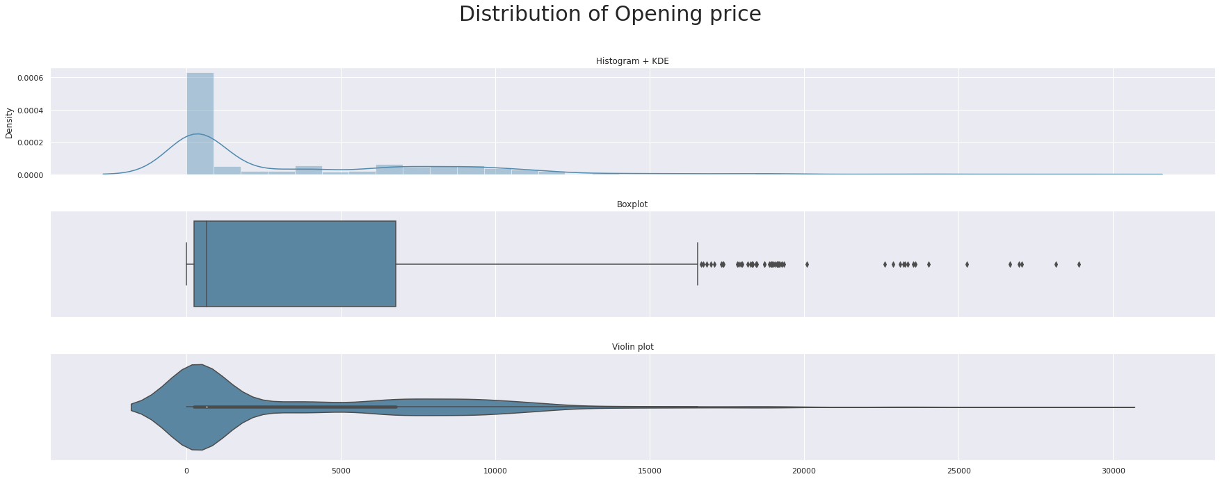
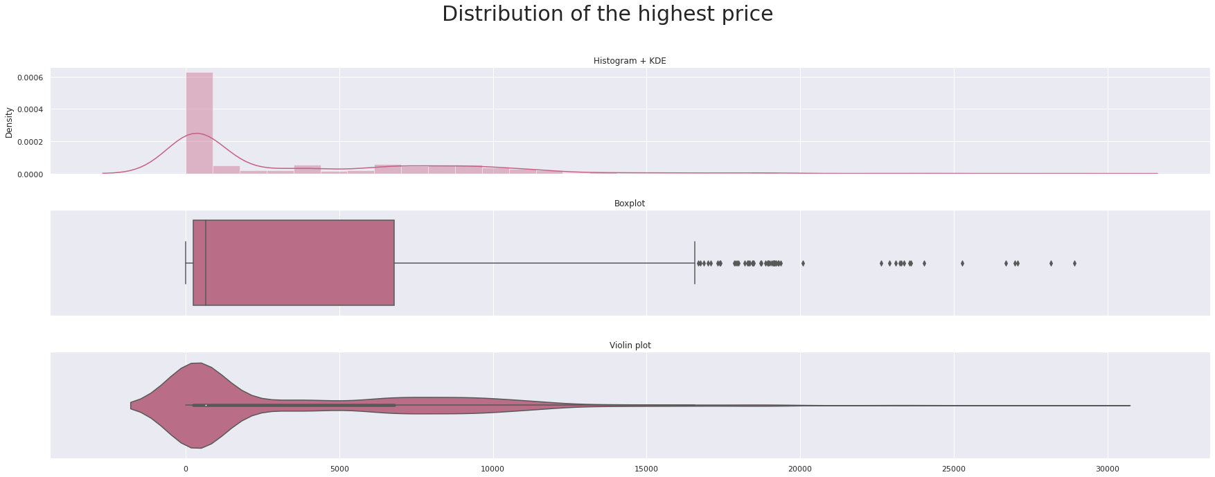
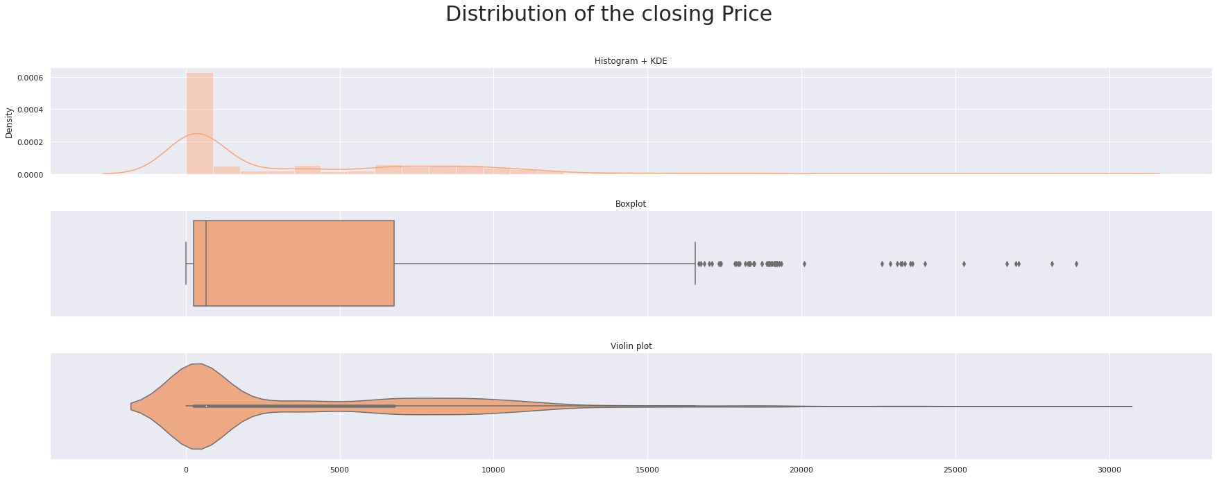
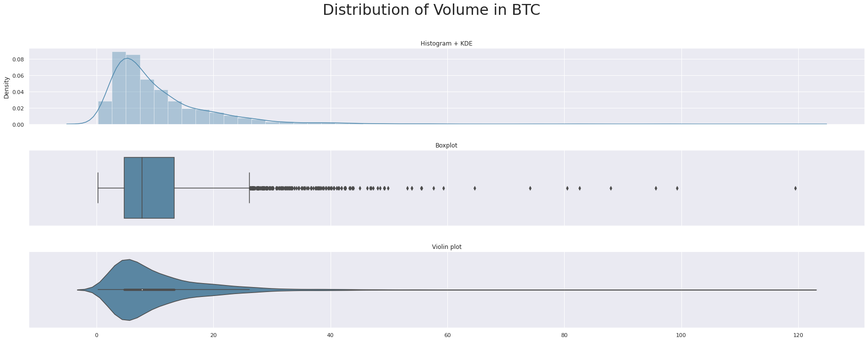
def triple_plot(x, title,c):
    fig, ax = plt.subplots(3,1,figsize=(25,10),sharex=True)
    sns.distplot(x, ax=ax[0],color=c)
    ax[0].set(xlabel=None)
    ax[0].set_title('Histogram + KDE')
    sns.boxplot(x, ax=ax[1],color=c)
    ax[1].set(xlabel=None)
    ax[1].set_title('Boxplot')
    sns.violinplot(x, ax=ax[2],color=c)
    ax[2].set(xlabel=None)
    ax[2].set_title('Violin plot')
    fig.suptitle(title, fontsize=30)
    plt.tight_layout(pad=3.0)
    plt.show()
triple_plot(data['Open'],'Distribution of Opening price',custom_colors[0])
triple_plot(data['High'],'Distribution of the highest price',custom_colors[1])
triple_plot(data['Low'],'Distribution of Lowest Price',custom_colors[2])

triple_plot(data['Close'],'Distribution of the closing Price',custom_colors[3])
triple_plot(data['Volume_(BTC)'],'Distribution of Volume in BTC ',custom_colors[0])
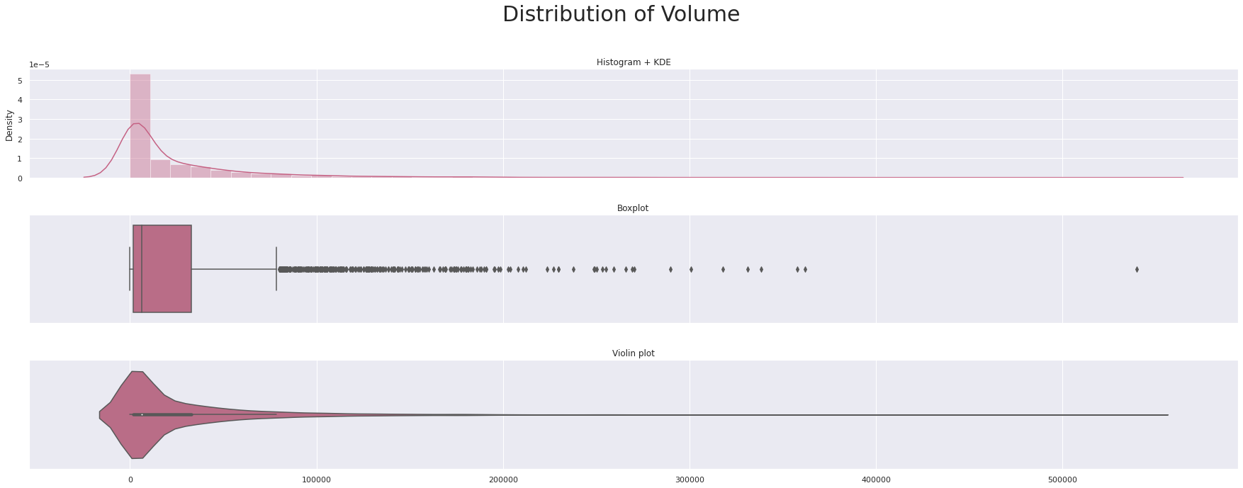
triple_plot(data['Volume_(Currency)'],'Distribution of Volume',custom_colors[1])
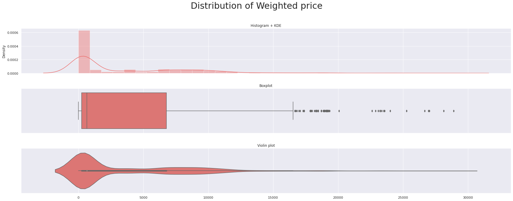
triple_plot(data['Weighted_Price'],'Distribution of Weighted price',custom_colors[2])
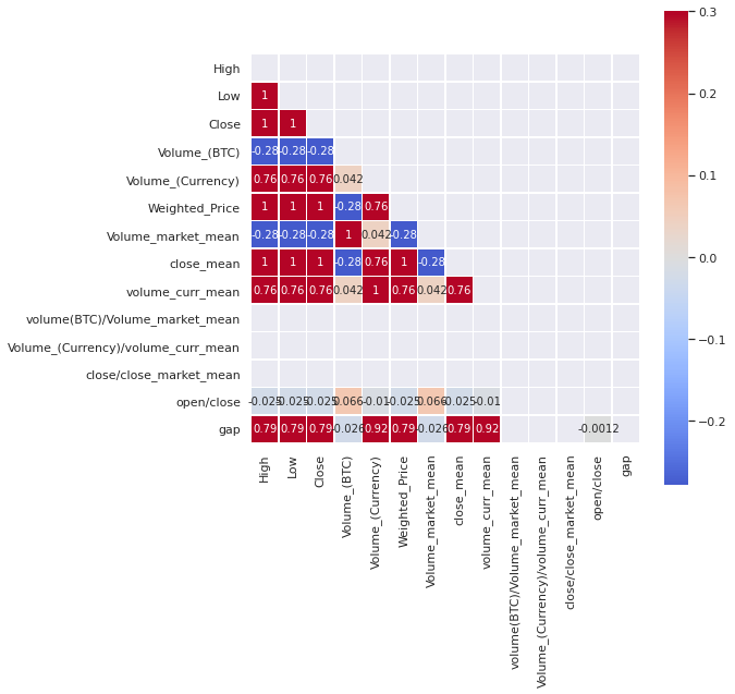
plt.figure(figsize=(8,8))
corr=data_df[data_df.columns[1:]].corr()
mask = np.triu(np.ones_like(corr, dtype=bool))
sns.heatmap(data_df[data_df.columns[1:]].corr(), mask=mask, cmap='coolwarm', vmax=.3, center=0,
            square=True, linewidths=.5,annot=True)
plt.show()
data_df=data_df.drop(columns=['volume(BTC)/Volume_market_mean','Volume_(Currency)/volume_curr_mean','close/close_market_mean'])
data_df.columns
Index(['Open', 'High', 'Low', 'Close', 'Volume_(BTC)', 'Volume_(Currency)',
       'Weighted_Price', 'Volume_market_mean', 'close_mean',
       'volume_curr_mean', 'open/close', 'gap'],
      dtype='object')
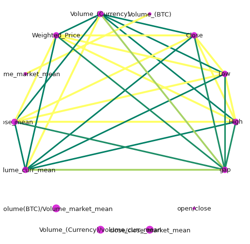
indices = corr.index.values
cor_matrix = np.asmatrix(corr)
G = nx.from_numpy_matrix(cor_matrix)
G = nx.relabel_nodes(G,lambda x: indices[x])
#G.edges(data=True)
def corr_network(G, corr_direction, min_correlation):
    H = G.copy()

    for s1, s2, weight in G.edges(data=True):
        if corr_direction == "positive":
            if weight["weight"] < 0 or weight["weight"] < min_correlation:
                H.remove_edge(s1, s2)
        else:
            if weight["weight"] >= 0 or weight["weight"] > min_correlation:
                H.remove_edge(s1, s2)

    edges,weights = zip(*nx.get_edge_attributes(H,'weight').items())
    weights = tuple([(1+abs(x))**2 for x in weights])

    d = dict(nx.degree(H))
    nodelist=d.keys()
    node_sizes=d.values()

    positions=nx.circular_layout(H)

    plt.figure(figsize=(9,9))

    nx.draw_networkx_nodes(H,positions,node_color='#d100d1',nodelist=nodelist,
                       node_size=tuple([x**2 for x in node_sizes]),alpha=0.8)

    nx.draw_networkx_labels(H, positions, font_size=13)

    if corr_direction == "positive":
        edge_colour = plt.cm.summer
    else:
        edge_colour = plt.cm.autumn

    nx.draw_networkx_edges(H, positions, edgelist=edges,style='solid',
                          width=weights, edge_color = weights, edge_cmap = edge_colour,
                          edge_vmin = min(weights), edge_vmax=max(weights))
    plt.axis('off')
    plt.show()
corr_network(G, corr_direction="positive",min_correlation = 0.5)

data_df.columns
Index(['Open', 'High', 'Low', 'Close', 'Volume_(BTC)', 'Volume_(Currency)',
       'Weighted_Price', 'Volume_market_mean', 'close_mean',
       'volume_curr_mean', 'open/close', 'gap'],
      dtype='object')
Time series Analysis and Prediction using Prophet

What is Prophet? Prophet is a facebooks’ open source time series prediction. Prophet decomposes time series into trend, seasonality and holiday. It has intuitive hyper parameters which are easy to tune.
things to note when using Prophet
- Accommodates seasonality with multiple periods
- Prophet is resilient to missing values
- Best way to handle outliers in Prophet is to remove them
- Fitting of the model is fast
- Intuitive hyper parameters which are easy to tune
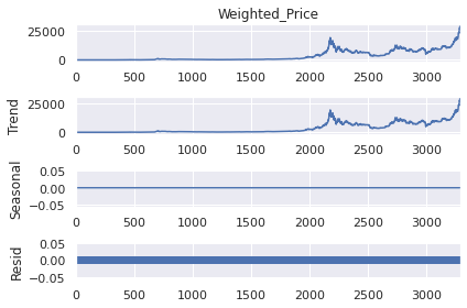
plt.figure(figsize=(15,12))
series = data_df.Weighted_Price
result = seasonal_decompose(series, model='additive',period=1)
result.plot()

<Figure size 1080x864 with 0 Axes>
# Renaming the column names accroding to Prophet's requirements
prophet_df=data_df[['Timestamp','Weighted_Price']]
prophet_df.rename(columns={'Timestamp':'ds','Weighted_Price':'y'},inplace=True)
/opt/conda/lib/python3.7/site-packages/pandas/core/frame.py:4446: SettingWithCopyWarning:


A value is trying to be set on a copy of a slice from a DataFrame

See the caveats in the documentation: https://pandas.pydata.org/pandas-docs/stable/user_guide/indexing.html#returning-a-view-versus-a-copy
prophet_basic = Prophet()
prophet_basic.fit(prophet_df[['ds','y']])
<fbprophet.forecaster.Prophet at 0x7ff8c52e7c10>
future= prophet_basic.make_future_dataframe(periods=365)#Making predictions for one year
future.tail(2)
| ds | |
|---|---|
| 3652 | 2021-12-30 |
| 3653 | 2021-12-31 |
forecast=prophet_basic.predict(future)
fig1 =prophet_basic.plot(forecast)
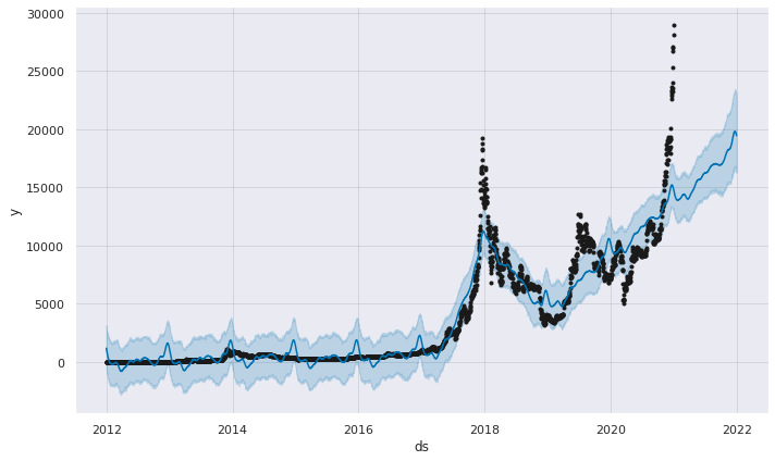
fig1 = prophet_basic.plot_components(forecast)
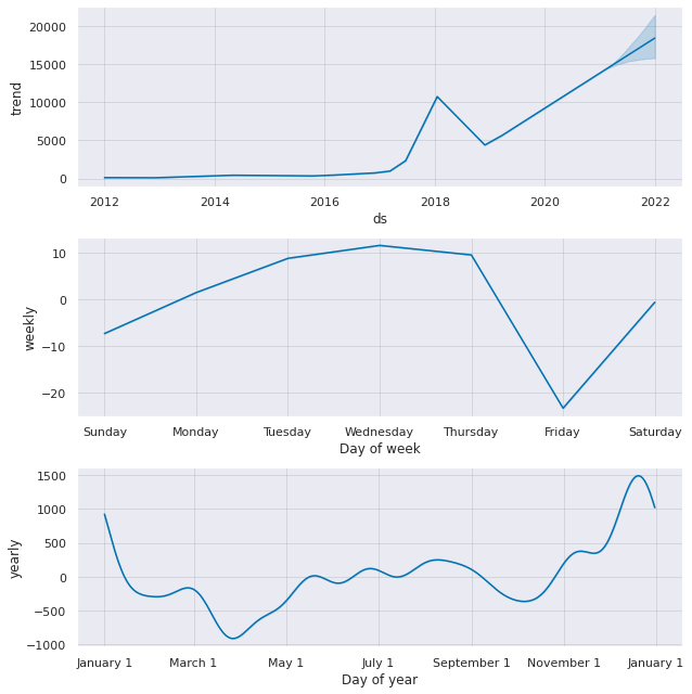
fig = prophet_basic.plot(forecast)
a = add_changepoints_to_plot(fig.gca(), prophet_basic, forecast)
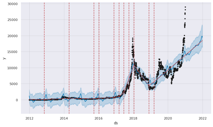
print(f'{m_}Change points:\n {y_}{prophet_basic.changepoints}\n')
[37mChange points:
[36m105 2012-04-14
210 2012-07-28
316 2012-11-11
421 2013-02-24
526 2013-06-09
631 2013-09-22
736 2014-01-05
842 2014-04-21
947 2014-08-04
1052 2014-11-17
1157 2015-03-02
1262 2015-06-15
1368 2015-09-29
1473 2016-01-12
1578 2016-04-26
1683 2016-08-09
1788 2016-11-22
1894 2017-03-08
1999 2017-06-21
2104 2017-10-04
2209 2018-01-17
2314 2018-05-02
2420 2018-08-16
2525 2018-11-29
2630 2019-03-14
Name: ds, dtype: datetime64[ns]
data_df.columns
Index(['Timestamp', 'Open', 'High', 'Low', 'Close', 'Volume_(BTC)',
       'Volume_(Currency)', 'Weighted_Price', 'Volume_market_mean',
       'close_mean', 'volume_curr_mean', 'open/close', 'gap', 'month'],
      dtype='object')
prophet_df['Open'] = data_df['Open']
prophet_df['High'] = data_df['High']
prophet_df['Low'] = data_df['Low']
prophet_df['Vol(BTC)'] = data_df['Volume_(BTC)']
prophet_df['Vol(curr)'] = data_df['Volume_(Currency)']
prophet_df['Volume_market_mean'] = data_df['Volume_market_mean']
prophet_df['close_mean'] = data_df['close_mean']
prophet_df['volume_curr_mean'] = data_df['volume_curr_mean']
prophet_df['open/close'] = data_df['open/close']
prophet_df['gap'] = data_df['gap']
/opt/conda/lib/python3.7/site-packages/ipykernel_launcher.py:1: SettingWithCopyWarning:


A value is trying to be set on a copy of a slice from a DataFrame.
Try using .loc[row_indexer,col_indexer] = value instead

See the caveats in the documentation: https://pandas.pydata.org/pandas-docs/stable/user_guide/indexing.html#returning-a-view-versus-a-copy

/opt/conda/lib/python3.7/site-packages/ipykernel_launcher.py:2: SettingWithCopyWarning:


A value is trying to be set on a copy of a slice from a DataFrame.
Try using .loc[row_indexer,col_indexer] = value instead

See the caveats in the documentation: https://pandas.pydata.org/pandas-docs/stable/user_guide/indexing.html#returning-a-view-versus-a-copy

/opt/conda/lib/python3.7/site-packages/ipykernel_launcher.py:3: SettingWithCopyWarning:


A value is trying to be set on a copy of a slice from a DataFrame.
Try using .loc[row_indexer,col_indexer] = value instead

See the caveats in the documentation: https://pandas.pydata.org/pandas-docs/stable/user_guide/indexing.html#returning-a-view-versus-a-copy

/opt/conda/lib/python3.7/site-packages/ipykernel_launcher.py:4: SettingWithCopyWarning:


A value is trying to be set on a copy of a slice from a DataFrame.
Try using .loc[row_indexer,col_indexer] = value instead

See the caveats in the documentation: https://pandas.pydata.org/pandas-docs/stable/user_guide/indexing.html#returning-a-view-versus-a-copy

/opt/conda/lib/python3.7/site-packages/ipykernel_launcher.py:5: SettingWithCopyWarning:


A value is trying to be set on a copy of a slice from a DataFrame.
Try using .loc[row_indexer,col_indexer] = value instead

See the caveats in the documentation: https://pandas.pydata.org/pandas-docs/stable/user_guide/indexing.html#returning-a-view-versus-a-copy

/opt/conda/lib/python3.7/site-packages/ipykernel_launcher.py:6: SettingWithCopyWarning:


A value is trying to be set on a copy of a slice from a DataFrame.
Try using .loc[row_indexer,col_indexer] = value instead

See the caveats in the documentation: https://pandas.pydata.org/pandas-docs/stable/user_guide/indexing.html#returning-a-view-versus-a-copy

/opt/conda/lib/python3.7/site-packages/ipykernel_launcher.py:7: SettingWithCopyWarning:


A value is trying to be set on a copy of a slice from a DataFrame.
Try using .loc[row_indexer,col_indexer] = value instead

See the caveats in the documentation: https://pandas.pydata.org/pandas-docs/stable/user_guide/indexing.html#returning-a-view-versus-a-copy

/opt/conda/lib/python3.7/site-packages/ipykernel_launcher.py:8: SettingWithCopyWarning:


A value is trying to be set on a copy of a slice from a DataFrame.
Try using .loc[row_indexer,col_indexer] = value instead

See the caveats in the documentation: https://pandas.pydata.org/pandas-docs/stable/user_guide/indexing.html#returning-a-view-versus-a-copy

/opt/conda/lib/python3.7/site-packages/ipykernel_launcher.py:9: SettingWithCopyWarning:


A value is trying to be set on a copy of a slice from a DataFrame.
Try using .loc[row_indexer,col_indexer] = value instead

See the caveats in the documentation: https://pandas.pydata.org/pandas-docs/stable/user_guide/indexing.html#returning-a-view-versus-a-copy

/opt/conda/lib/python3.7/site-packages/ipykernel_launcher.py:10: SettingWithCopyWarning:


A value is trying to be set on a copy of a slice from a DataFrame.
Try using .loc[row_indexer,col_indexer] = value instead

See the caveats in the documentation: https://pandas.pydata.org/pandas-docs/stable/user_guide/indexing.html#returning-a-view-versus-a-copy
pro_regressor= Prophet()
pro_regressor.add_regressor('Open')
pro_regressor.add_regressor('High')
pro_regressor.add_regressor('Low')
pro_regressor.add_regressor('Vol(BTC)')
pro_regressor.add_regressor('Vol(curr)')
pro_regressor.add_regressor('Volume_market_mean')
pro_regressor.add_regressor('close_mean')
pro_regressor.add_regressor('volume_curr_mean')
pro_regressor.add_regressor('open/close')
pro_regressor.add_regressor('gap')

train_X= prophet_df[:2500]
test_X= prophet_df[2500:]
#Fitting the data
pro_regressor.fit(train_X)
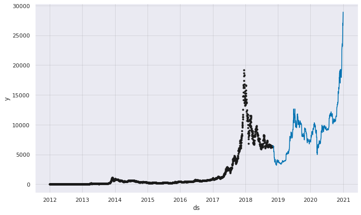
future_data = pro_regressor.make_future_dataframe(periods=249)
#Forecast the data for Test  data
forecast_data = pro_regressor.predict(test_X)
pro_regressor.plot(forecast_data);
6 different types of metrics are shown by each time horizon, but by taking moving average over 37 days in this case (can be changed by ‘rolling_window’ option).
df_cv = cross_validation(pro_regressor, initial='100 days', period='180 days', horizon = '365 days')
pm = performance_metrics(df_cv, rolling_window=0.1)
display(pm.head(),pm.tail())
fig = plot_cross_validation_metric(df_cv, metric='mape', rolling_window=0.1)
plt.show()
0%| | 0/12 [00:00<?, ?it/s]
| horizon | mse | rmse | mae | mape | mdape | coverage | |
|---|---|---|---|---|---|---|---|
| 0 | 37 days | 0.413771 | 0.643251 | 0.216705 | 0.001091 | 0.000171 | 0.785388 |
| 1 | 38 days | 0.469662 | 0.685319 | 0.231994 | 0.001188 | 0.000175 | 0.779680 |
| 2 | 39 days | 0.539967 | 0.734825 | 0.249433 | 0.001294 | 0.000178 | 0.772831 |
| 3 | 40 days | 0.615809 | 0.784735 | 0.268262 | 0.001407 | 0.000180 | 0.767123 |
| 4 | 41 days | 0.688987 | 0.830052 | 0.286306 | 0.001525 | 0.000188 | 0.764840 |
| horizon | mse | rmse | mae | mape | mdape | coverage | |
|---|---|---|---|---|---|---|---|
| 324 | 361 days | 23.897097 | 4.888466 | 1.934879 | 0.006200 | 0.000758 | 0.849315 |
| 325 | 362 days | 23.913066 | 4.890099 | 1.935748 | 0.006199 | 0.000381 | 0.851598 |
| 326 | 363 days | 23.928062 | 4.891632 | 1.936313 | 0.006196 | 0.000713 | 0.853881 |
| 327 | 364 days | 23.944867 | 4.893349 | 1.935958 | 0.006192 | 0.000586 | 0.856164 |
| 328 | 365 days | 23.963754 | 4.895279 | 1.936640 | 0.006186 | 0.000557 | 0.858447 |
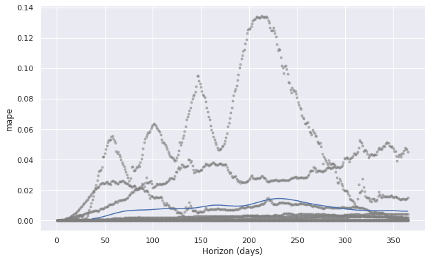
The MAPE (Mean Absolute Percent Error) measures the size of the error in percentage terms. It is calculated as the average of the unsigned percentage error Many organizations focus primarily on the MAPE when assessing forecast accuracy. Most people are comfortable thinking in percentage terms, making the MAPE easy to interpret. It can also convey information when you don’t know the item’s demand volume. For example, telling your manager, “we were off by less than 4%” is more meaningful than saying “we were off by 3,000 cases,” if your manager doesn’t know an item’s typical demand volume.
What Prophet doesnt do
- Prophet does not allow non-Gaussian noise distribution: In Prophet, noise distribution is always Gaussian and pre-transformation of y values is the only way to handle the values following skewed distribution.
- Prophet does not take autocorrelation on residual into account Since epsilon noise portion in the formula assume i.i.d. normal distribution, the residual is not assumed to have autocorrelation, unlike ARIMA model.
- Prophet does not assume stochastic trend Prophet’s trend component is always deterministic+possible changepoints and it won’t assume stochastic trend unlike ARIMA.